Here we are going to explore Machine Learning with Tidymodels on the ERA agroforestry data
Loading necessary R packages and ERA data
Loading general R packages
This part of the document is where we actually get to the nitty-gritty of the ERA agroforestry data and therefore it requires us to load a number of R packages for both general Explorortive Data Analysis and Machine Learning.
Show code
# Using the pacman functions to load required packages
if(!require("pacman", character.only = TRUE)){
install.packages("pacman",dependencies = T)
}
# ------------------------------------------------------------------------------------------
# General packages
# ------------------------------------------------------------------------------------------
required.packages <- c("tidyverse", "here", "see", "ggplot2", "hablar", "kableExtra", "RColorBrewer",
"cowplot", "ggpubr", "ggbeeswarm", "viridis", "GGally", "DataExplorer", "corrr",
"ggridges", "Boruta",
# ------------------------------------------------------------------------------------------
# Parallel computing packages
# ------------------------------------------------------------------------------------------
"parallelMap", "parallelly", "parallel",
# ------------------------------------------------------------------------------------------
# Packages specifically for tidymodels machine learning
# ------------------------------------------------------------------------------------------
"tidymodels", "treesnip","stacks", "workflowsets",
"finetune", "vip", "modeldata", "finetune",
"visdat", "spatialsample", "kknn",
"kernlab", "ranger", "xgboost", "tidyposterior"
)
p_load(char=required.packages, install = T,character.only = T)
Loading the ERAg package
The ERAg package includes all the ERA data we need for our ED steps.
Show code
# devtools::install_github("peetmate/ERAg",
# auth_token = "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",
# build_vignettes = T)
library(ERAg)
Preliminary data cleaning and data wrangling
The real power of ERA is that it is geo-referenced by latitude and longitude of where the agricultural research/study was performed. This make it exceptionally relevant for getting insights into useful relationships between any spatially explicit data and ERA practices, outcomes and (crop) products. Any data that can be spatially referenced such as weather, soil, marked access etc. can be investigated in relation to ERA data. In our case we are going to make use of two datasets, a digital soil for the continent of Africa called iSDA and a climate dataset, called BioClim adapted from WorldClim.org to have more biologically meaningful variables. The digital soil map on 30 m resolution is from the Innovative Solutions for Decision Agriculture (iSDA) data from Hengl, T., Miller, M.A.E., Križan, J. et al. (2021). Please see the websites isda-africa.com, worldagroforestry.org/isda and zenodo.org/isdasoil for more information and direct data access to this soil data. Please see the paper of Noce, S., Caporaso, L. & Santini, M. (2020) for more information on WorldClim and BioClim variables.
Merging ERA and biophysical pretictor features
Now that we are familiar with the biophysical co-variables, we are going to merging our ERA agroforestry data with the iSDA and the BioClim data. We can use the coordinate information we have from our latitude and longitude columns in our ERA agroforestry data to merge by.
Note: here that we are proceeding with the agroforestry dataset called “ERA.AF.PR.TRESH” that we created in the previous section - because this dataset is the subset of ERA.Compiled, in which we have only agroforestry data, we have filtered out all non-annual crops and included a thresholds with a minimum of 25 observations per agroforestry practice. The ERA.AF.PR.TRESH data is not the output of the ERAg::PrepareERA function, thus we have not removed data with negative outcomes, that would potentially cause issues in the machine learning analysis.
BioClim climate co-variables
Show code
# Getting the BioClim co-variables from the ERAg package and converting the dataset to a dataframe
ERA.BioClim <- as.data.table(ERAg::ERA_BioClim)
# Changing the name of the column that contains the coordinates from "V1" to "Site.Key", so that we can use it to merge later
names(ERA.BioClim)[names(ERA.BioClim) == "V1"] <- "Site.Key"
# ------------------------------------------------------------------------------------------------------------------------
# merging with the agroforestry.bioclim data using the common "Site.Key" coordinates and creating a new dataset
era.agrofor.bioclim <- cbind(era.agrofor, ERA.BioClim[match(era.agrofor[, Site.Key], ERA.BioClim[, Site.Key])])
dim(era.agrofor.bioclim)
# [1] 6361 332
# rmarkdown::paged_table(era.agrofor.bioclim)
ERA Physical co-variables
Show code
# Getting some of the older the physical (ERA_Physical) co-variables from the ERAg package.
# Note that we load in this ERA data because some of this information is not found in the iSDA data (e.g. altitude and slope)
#converting the dataset to a dataframe
ERA.Phys <- as.data.table(ERAg::ERA_Physical)
# selecting features
ERA.Phys <- ERA.Phys %>%
dplyr::select(Site.Key, Altitude.mean, Altitude.sd, Altitude.max, Altitude.min, Slope.med, Slope.mean, Slope.sd, Slope.max,
Slope.min, Aspect.med, Aspect.mean, Aspect.sd)
# ------------------------------------------------------------------------------------------------------------------------
# merging with the era.agrofor.bioclim data using the common "Site.Key" coordinates and creating a new dataset
era.agrofor.bioclim.phys <- cbind(era.agrofor.bioclim, ERA.Phys[match(era.agrofor.bioclim[, Site.Key], ERA.Phys[, Site.Key])])
dim(era.agrofor.bioclim.phys)
# [1] 6361 345
iSDA soil co-variables In a similar fasion we can load the iSDA soil co-variables from the ERAg package.
Show code
# iSDA
iSDAsoils <- ERAg::ERA_ISDA
# We want to retain the soil depth information from iSDA, so we create fields for upper and lower measurement depths.
iSDAsoils[grepl("0..200cm",Variable),Depth.Upper:=0
][grepl("0..200cm",Variable),Depth.Lower:=200
][,Variable:=gsub("_m_30m_0..200cm","",Variable)]
iSDAsoils[grepl("0..20cm",Variable),Depth.Upper:=0
][grepl("0..20cm",Variable),Depth.Lower:=20
][,Variable:=gsub("_m_30m_0..20cm","",Variable)]
iSDAsoils[grepl("20..50cm",Variable),Depth.Upper:=20
][grepl("20..50cm",Variable),Depth.Lower:=50
][,Variable:=gsub("_m_30m_20..50cm","",Variable)]
iSDAsoils[,Weight:=Depth.Lower-Depth.Upper]
iSDAsoils <- unique(iSDAsoils[,list(Median=weighted.mean(Median,Weight),Mean=weighted.mean(Mean,Weight),SD=weighted.mean(SD,Weight),Mode=Mode[Weight==max(Weight)]),by=list(Variable,Site.Key)])
iSDAsoils <- dcast(iSDAsoils,Site.Key~Variable,value.var = c("Median","Mean","SD","Mode"))
ERA.iSDA <- as.data.table(iSDAsoils)
# ------------------------------------------------------------------------------------------------------------------------
# merging with the era.agrofor.bioclim.phys data using the common "Site.Key" coordinates and creating a new dataset
era.agrofor.bioclim.phys.isda <- cbind(era.agrofor.bioclim.phys, ERA.iSDA[match(era.agrofor.bioclim.phys[, Site.Key], ERA.iSDA[, Site.Key])])
dim(era.agrofor.bioclim.phys.isda)
# [1] 6361 425
# ([1] 6361 418)
We see that the number of features have increased dramatically. We now have 418 co-variables, also called independent variables in modelling, and features in typical machine learning language. From now on the term “feature” will be used to describe the columns including the co-variables.
Removing duplicated columns
Show code
era.agrofor.bioclim.phys.isda.no.dubl <- era.agrofor.bioclim.phys.isda %>%
subset(., select = which(!duplicated(names(.))))
Data Cleaning
Deriving value from any machine learning-based approach crucially depends on the quality of the underlying data. There is a lot of data wrangling and pre-processing to do before this messy data is useful and ready for machine learning analysis. We are first going to perform some preliminary data cleaning as our first pre-processing step. Even though many of the important data cleaning steps are integrated into the tidymodels framework when we are going to construct our machine learning model workflows it is still important to perform the crucial data cleaning step manually prior to advancing into the more complex machine learning in order to get a better understanding of the nature of the data.
We will iterate between the data cleaning and the exploitative data analysis of the agroforestry data.
Renaming features from BioClim and iSDA Note that all variables are mean values. Keep individual units in mind!
# New ERA dataframe with all biophysical co-variables
agrofor.biophys <- data.table::copy(era.agrofor.bioclim.phys.isda.no.dubl)
dim(era.agrofor.bioclim.phys.isda.no.dubl)
# [1] 6361 415
class(agrofor.biophys)
# [1] "data.table" "data.frame"
dim(agrofor.biophys)
# [1] 6361 415
agrofor.biophys.rename <- data.table::copy(agrofor.biophys) %>%
# Renaming BioClim features
rename(Bio01_MT_Annu = wc2.1_30s_bio_1.Mean) %>%
rename(Bio02_MDR = wc2.1_30s_bio_2.Mean) %>%
rename(Bio03_Iso = wc2.1_30s_bio_3.Mean) %>%
rename(Bio04_TS = wc2.1_30s_bio_4.Mean) %>%
rename(Bio05_TWM = wc2.1_30s_bio_5.Mean) %>%
rename(Bio06_MinTCM = wc2.1_30s_bio_6.Mean) %>%
rename(Bio07_TAR = wc2.1_30s_bio_7.Mean) %>%
rename(Bio08_MT_WetQ = wc2.1_30s_bio_8.Mean) %>%
rename(Bio09_MT_DryQ = wc2.1_30s_bio_9.Mean) %>%
rename(Bio10_MT_WarQ = wc2.1_30s_bio_10.Mean) %>%
rename(Bio11_MT_ColQ = wc2.1_30s_bio_11.Mean) %>%
rename(Bio12_Pecip_Annu = wc2.1_30s_bio_12.Mean) %>%
rename(Bio13_Precip_WetM = wc2.1_30s_bio_13.Mean) %>%
rename(Bio14_Precip_DryM = wc2.1_30s_bio_14.Mean) %>%
rename(Bio15_Precip_S = wc2.1_30s_bio_15.Mean) %>%
rename(Bio16_Precip_WetQ = wc2.1_30s_bio_16.Mean) %>%
rename(Bio17_Precip_DryQ = wc2.1_30s_bio_17.Mean) %>%
rename(Bio18_Precip_WarQ = wc2.1_30s_bio_18.Mean) %>%
rename(Bio19_Precip_ColQ = wc2.1_30s_bio_19.Mean) %>%
# Renaming iSDA soil variables
rename(iSDA_Depth_to_bedrock = Mean_bdr) %>%
rename(iSDA_SAND_conc = Mean_sand_tot_psa) %>%
rename(iSDA_SILT_conc = Mean_silt_tot_psa) %>%
rename(iSDA_CLAY_conc = Mean_clay_tot_psa) %>%
rename(iSDA_FE_Bulk_dens = Mean_db_od) %>%
rename(iSDA_log_C_tot = Mean_log.c_tot) %>%
rename(iSDA_log_Ca = Mean_log.ca_mehlich3) %>%
rename(iSDA_log_eCEC = Mean_log.ecec.f) %>%
rename(iSDA_log_Fe = Mean_log.fe_mehlich3) %>%
rename(iSDA_log_K = Mean_log.k_mehlich3) %>%
rename(iSDA_log_Mg = Mean_log.mg_mehlich3) %>%
rename(iSDA_log_N = Mean_log.n_tot_ncs) %>%
rename(iSDA_log_SOC = Mean_log.oc) %>%
rename(iSDA_log_P = Mean_log.p_mehlich3) %>%
rename(iSDA_log_S = Mean_log.s_mehlich3) %>%
rename(iSDA_pH = Mean_ph_h2o) %>%
# Renaming iSDA soil texture values based on the guide according to iSDA
rowwise() %>%
mutate(Texture_class_20cm_descrip =
case_when(
as.numeric(Mode_texture.class) == 1 ~ "Clay",
as.numeric(Mode_texture.class) == 2 ~ "Silty_clay",
as.numeric(Mode_texture.class) == 3 ~ "Sandy_clay",
as.numeric(Mode_texture.class) == 4 ~ "Loam",
as.numeric(Mode_texture.class) == 5 ~ "Silty_clay_loam",
as.numeric(Mode_texture.class) == 6 ~ "Sandy_clay_loam",
as.numeric(Mode_texture.class) == 7 ~ "Loam",
as.numeric(Mode_texture.class) == 8 ~ "Silt_loam",
as.numeric(Mode_texture.class) == 9 ~ "Sandy_loam",
as.numeric(Mode_texture.class) == 10 ~ "Silt",
as.numeric(Mode_texture.class) == 11 ~ "Loam_sand",
as.numeric(Mode_texture.class) == 12 ~ "Sand",
as.numeric(Mode_texture.class) == 255 ~ "NODATA")) %>%
# Renaming the ASTER variables, slope and elevation
rename(ASTER_Slope = Slope.mean) %>%
rename(ASTER_Altitude = Altitude.mean) %>%
# Renaming agroecological zone 16 simple
mutate(AEZ16s = AEZ16simple)
# Error: C stack usage 7969312 is too close to the limit
Fixing empty cells in the Tree column
Show code
agrofor.biophys.rename <- agrofor.biophys.rename %>%
#dplyr::filter_all(all_vars(!is.infinite(.))) %>%
dplyr::mutate(across(Tree, ~ ifelse(. == "", NA, as.character(.)))) %>%
mutate_if(is.character, factor) %>%
dplyr::mutate(across(Tree, ~ ifelse(. == "NA", "Unknown_tree", as.character(.)))) %>%
dplyr::mutate(across(AEZ16s, ~ ifelse(. == "NA", "Unknown_AEZ16", as.character(.)))) %>%
replace_na(list(Tree = "Unknown_Tree", AEZ16s = "Unknown_AEZ16s"))
# Error: C stack usage 7969312 is too close to the limit
There are currently several site types we will change this so we only have three site types. A Site.Type called “Farm,” another called “Station” and a third one called “Other,” that will collect site types that are neither Farm nor Station. We will also remove the site type “Greenhouse,” as it does not make sense in an agroforestry setting. It remains unknown where the ERA agroforestry observations with “Greenhouse” as site type come from..
Renaming the column Site.Types
Selecting ERA Agroforestry outcomes; Crop and Biomass Yield
For this machine learning analysis we will only focus on agroforestry data that have crop and biomass yield as outcomes. This is because it is not meaningful to compare response ratios across the diverse set of ERA outcomes as the basis for calculating MeanC and MeanT might vary tremendously. Hence due to that fact we are subsetting on Out.SubInd for crop and biomass yield.
agrofor.biophys.outcome.yield <- agrofor.biophys.rename %>%
dplyr::filter(Out.SubInd == "Crop Yield" | Out.SubInd == "Biomass Yield")
Selecting features for modelling and calculating outcome variable, response ratios
we are going to select the features for our modelling and machine learning exercise. We are selecting MeanC and MeanT as we will convert these to one outcome feature.
Selecting feature columns for modelling
agrofor.biophys.selected.features <- data.table::copy(agrofor.biophys.outcome.yield) %>%
dplyr::select(MeanC, # Outcome variable(s)
MeanT,
ID, # ID variable (will not be included as predictor)
AEZ16s, # ID variable (will not be included as predictor)
PrName, # ID variable (will not be included as predictor)
PrName.Code, # ID variable (will not be included as predictor)
SubPrName, # ID variable (will not be included as predictor)
Product, # ID variable (will not be included as predictor)
Out.SubInd, # ID variable (will not be included as predictor)
Out.SubInd.Code, # ID variable (will not be included as predictor)
Country, # ID variable (will not be included as predictor)
Latitude, # ID variable (will not be included as predictor, but as a basis for the spatial/cluster cross-validation)
Longitude, # ID variable (will not be included as predictor, but as a basis for the spatial/cluster cross-validation)
Site.Type, # Site_Type will be included as predictor, to see how much it explains the outcome
Tree, # Tree will be included as predictor, to see how much it explains the outcome
Bio01_MT_Annu,
Bio02_MDR,
Bio03_Iso,
Bio04_TS,
Bio05_TWM,
Bio06_MinTCM,
Bio07_TAR,
Bio08_MT_WetQ,
Bio09_MT_DryQ,
Bio10_MT_WarQ,
Bio11_MT_ColQ,
Bio12_Pecip_Annu,
Bio13_Precip_WetM,
Bio14_Precip_DryM,
Bio15_Precip_S,
Bio16_Precip_WetQ,
Bio17_Precip_DryQ,
iSDA_Depth_to_bedrock,
iSDA_SAND_conc,
iSDA_CLAY_conc,
iSDA_SILT_conc,
iSDA_FE_Bulk_dens,
iSDA_log_C_tot,
iSDA_log_Ca,
iSDA_log_eCEC,
iSDA_log_Fe,
iSDA_log_K,
iSDA_log_Mg,
iSDA_log_N,
iSDA_log_SOC,
iSDA_log_P,
iSDA_log_S,
iSDA_pH,
ASTER_Altitude,
ASTER_Slope
) %>%
relocate(ID, PrName, Out.SubInd, Product, AEZ16s, Country, Site.Type, MeanC, MeanT, Tree)
dim(agrofor.biophys.selected.features)
# [1] 4578 48
class(agrofor.biophys.selected.features)
# [1] "rowwise_df" "tbl_df" "tbl" "data.frame"
Calculating response ratios for each observation
We are going to compute a simple response ratio as RR = (MeanT/MeanC) and a log-transformed response ratio as logRR = (log(MeanT/MeanC)). The later will be used as our outcome variable.
agrofor.biophys.modelling.data <- data.table::copy(agrofor.biophys.selected.features) %>%
#subset(., select = which(!duplicated(names(.)))) %>% # First, removing duplicated columns
dplyr::mutate(RR = (MeanT/MeanC)) %>%
dplyr::mutate(logRR = (log(MeanT/MeanC)))
dim(agrofor.biophys.modelling.data)
# [1] 4578 52
Lets have a look at our modelling data with selected features and our outcome, calculated response ratios
Show code
agrofor.biophys.modelling.data <- readRDS(file = here::here("TidyMod_OUTPUT","agrofor.biophys.modelling.data.RDS"))
rmarkdown::paged_table(agrofor.biophys.modelling.data)
Show code
agrofor.biophys.modelling.data %>% group_by()
# A tibble: 4,578 × 52
ID PrName Out.SubInd Product AEZ16s Country Site.Type MeanC
<dbl> <fct> <fct> <fct> <fct> <fct> <fct> <dbl>
1 1660 Parklands Biomass Yi… Pearl … Warm.… Niger Farm 3.45
2 1660 Parklands Biomass Yi… Pearl … Warm.… Niger Farm 4.55
3 1675 Agrofores… Biomass Yi… Pearl … Warm.… Niger Farm 2.20
4 1675 Agrofores… Biomass Yi… Pearl … Warm.… Niger Farm 2.20
5 1675 Agrofores… Biomass Yi… Pearl … Warm.… Niger Farm 2.20
6 1675 Agrofores… Biomass Yi… Pearl … Warm.… Niger Farm 4.14
7 1675 Agrofores… Biomass Yi… Pearl … Warm.… Niger Farm 5.46
8 1675 Agrofores… Biomass Yi… Pearl … Warm.… Niger Farm 5.46
9 1675 Agrofores… Crop Yield Pearl … Warm.… Niger Farm 0.577
10 1675 Agrofores… Crop Yield Pearl … Warm.… Niger Farm 0.577
# … with 4,568 more rows, and 44 more variables: MeanT <dbl>,
# Tree <fct>, PrName.Code <fct>, SubPrName <fct>,
# Out.SubInd.Code <fct>, Latitude <dbl>, Longitude <dbl>,
# Bio01_MT_Annu <dbl>, Bio02_MDR <dbl>, Bio03_Iso <dbl>,
# Bio04_TS <dbl>, Bio05_TWM <dbl>, Bio06_MinTCM <dbl>,
# Bio07_TAR <dbl>, Bio08_MT_WetQ <dbl>, Bio09_MT_DryQ <dbl>,
# Bio10_MT_WarQ <dbl>, Bio11_MT_ColQ <dbl>, …Looks pretty good, however we have many empty cells for the Tree column that needs to be fixed. We have a data.frame (rowwise_df, tbl_df, tbl, data.frame) with 4578 observations and 52 features. Four of these features are our MeanC and MeanT that we will use to calculate the response ratio (RR and logRR). The RR and/or logRR will be our outcome feature, also called response variable. Hence, we have 52 - (4 + 11) = 37 predictors of which 35 are numeric and two (Tree and Site.Type are categorical/factors).
Creating data with only numeric predictors
A separate dataset with only numeric predictors and our outcome (RR and logRR) can be helpful when performing some important exploitative data analysis.
agrofor.biophys.modelling.data.numeric <- data.table::copy(agrofor.biophys.modelling.data) %>%
dplyr::select(RR,
logRR,
Bio01_MT_Annu,
Bio02_MDR,
Bio03_Iso,
Bio04_TS,
Bio05_TWM,
Bio06_MinTCM,
Bio07_TAR,
Bio08_MT_WetQ,
Bio09_MT_DryQ,
Bio10_MT_WarQ,
Bio11_MT_ColQ,
Bio12_Pecip_Annu,
Bio13_Precip_WetM,
Bio14_Precip_DryM,
Bio15_Precip_S,
Bio16_Precip_WetQ,
Bio17_Precip_DryQ,
iSDA_Depth_to_bedrock,
iSDA_SAND_conc,
iSDA_CLAY_conc,
iSDA_SILT_conc,
iSDA_FE_Bulk_dens,
iSDA_log_C_tot,
iSDA_log_Ca,
iSDA_log_eCEC,
iSDA_log_Fe,
iSDA_log_K,
iSDA_log_Mg,
iSDA_log_N,
iSDA_log_SOC,
iSDA_log_P,
iSDA_log_S,
iSDA_pH,
ASTER_Altitude,
ASTER_Slope
)
Explorotive Data Analysis
We are going to perform some exploratory data analysis (EDA) of the ERA agroforestry data. EDA is a critical pre-modelling step in order to make initial investigations so as to discover patterns, to spot anomalies, test hypothesis and to check assumptions. We are going to do this on the agroforestry data with the help of visualisations and summary statistics. Performing exploratory data analysis prior to conducting any machine learning is always a good idea, as it will help to get an understanding of the data in terms of relationships and how different predictor features are distributed, how they relate to the outcome (logRR) and how they relate to each other. Explorative data analysis is often an iterative process consisting of posing a question to the data, review the data, and develop further questions to investigate it before beginning the modelling and machine learning development. Hence, we need to conduct a proper EDA of our agroforestry data as it is fundamental to our later machine learning-based modelling analysis. We will first visually explore our agroforestry data using the DataExplorer package to generate histograms, density plots and scatter plots of the biophysical predictors. We will examine the results critically with our later machine learning approach in mind. We will continue the EDA by looking at the correlations between our biophysical predictors - and between our predictors and the outcome (logRR) to see if we can make any initial pattern recognition manually. Overall we will use the outcome of our EDA to identify required pre-processing steps needed for our machine learning models (e.g. excluding highly correlated predictors or normalizing some features for better model performance).
We will go through these nine steps in the EDA:
1) Missing data exploration
2) Density distributions of features i) of continuous predictors (all biophysical) i) of outcome (RR and logRR)
3) Histograms of features
- of continuous predictors (all biophysical)
- of outcome (RR and logRR)
4) Scatter plots
- of continuous predictors (all biophysical)
- of outcome (RR and logRR)
5) Quantile-quantile plots
- of continuous predictors (all biophysical)
- of outcome (RR and logRR)
6) Discritization of target feature, logRR
- Boxplots of predictors vs. discritized logRR**
7) PCA and variable importance
- of continuous predictors (all biophysical)
8) Correlation of features
- of numeric predictors (all biophysical)
- of outcome (RR and logRR)
9) Multiple pairwise t-test using discritized logRR values
- of continuous predictors (all biophysical)
Lets first familiarise ourself with the agroforestry data using the functions introduce() and plot_intro() from DataExplorer package.
Show code
DataExplorer::introduce(agrofor.biophys.modelling.data) %>% glimpse()
Rows: 1
Columns: 9
Rowwise:
$ rows <int> 4578
$ columns <int> 52
$ discrete_columns <int> 10
$ continuous_columns <int> 42
$ all_missing_columns <int> 0
$ total_missing_values <int> 2436
$ complete_rows <int> 4473
$ total_observations <int> 238056
$ memory_usage <dbl> 1783016Show code
DataExplorer::plot_intro(agrofor.biophys.modelling.data)
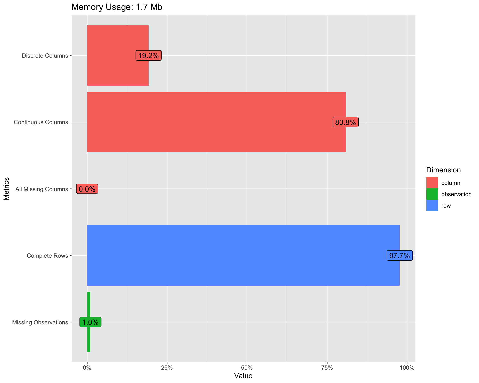
(#fig:Re-introduction to the agroforestry data plot)Re-introducing the agroforestry data
Missing data exploration
As part of the EDA of data cleaning we would need to deal with missing data in our agroforestry data. To get a better understanding of our missing data, such as “where it is” and how it manifest it self. We are going to make use of the naniar package, that is excellent for familiarixing our selfs with the missingness of the data.
First, lets view the number and percentage of missing values in each combination of grouped levels of practices (PrName) and outcomes (Out.SubInd).
Show code
agrofor.biophys.modelling.data.missing <- agrofor.biophys.modelling.data %>%
dplyr::group_by(PrName, Out.SubInd, AEZ16s) %>%
naniar::miss_var_summary() %>%
arrange(desc(n_miss))
Show code
rmarkdown::paged_table(agrofor.biophys.modelling.data.missing)
Now we can visually assess where there is missing data. Lets also make one where we facet based on agroecological zones as it is interesting to see in which agroecological zones we miss data.
agrofor.biophys.gg_miss_var.all <- naniar::gg_miss_var(agrofor.biophys.modelling.data,
show_pct = TRUE,
facet = "none")
agrofor.biophys.gg_miss_var.AEZ <- naniar::gg_miss_var(agrofor.biophys.modelling.data,
show_pct = TRUE,
facet = AEZ16s)
# Warning: It is deprecated to specify `guide = FALSE` to remove a guide. Please use `guide = "none"` instead.
Show code
agrofor.biophys.gg_miss_var.combined <- cowplot::plot_grid(agrofor.biophys.gg_miss_var.all,
agrofor.biophys.gg_miss_var.AEZ)
agrofor.biophys.gg_miss_var.combined
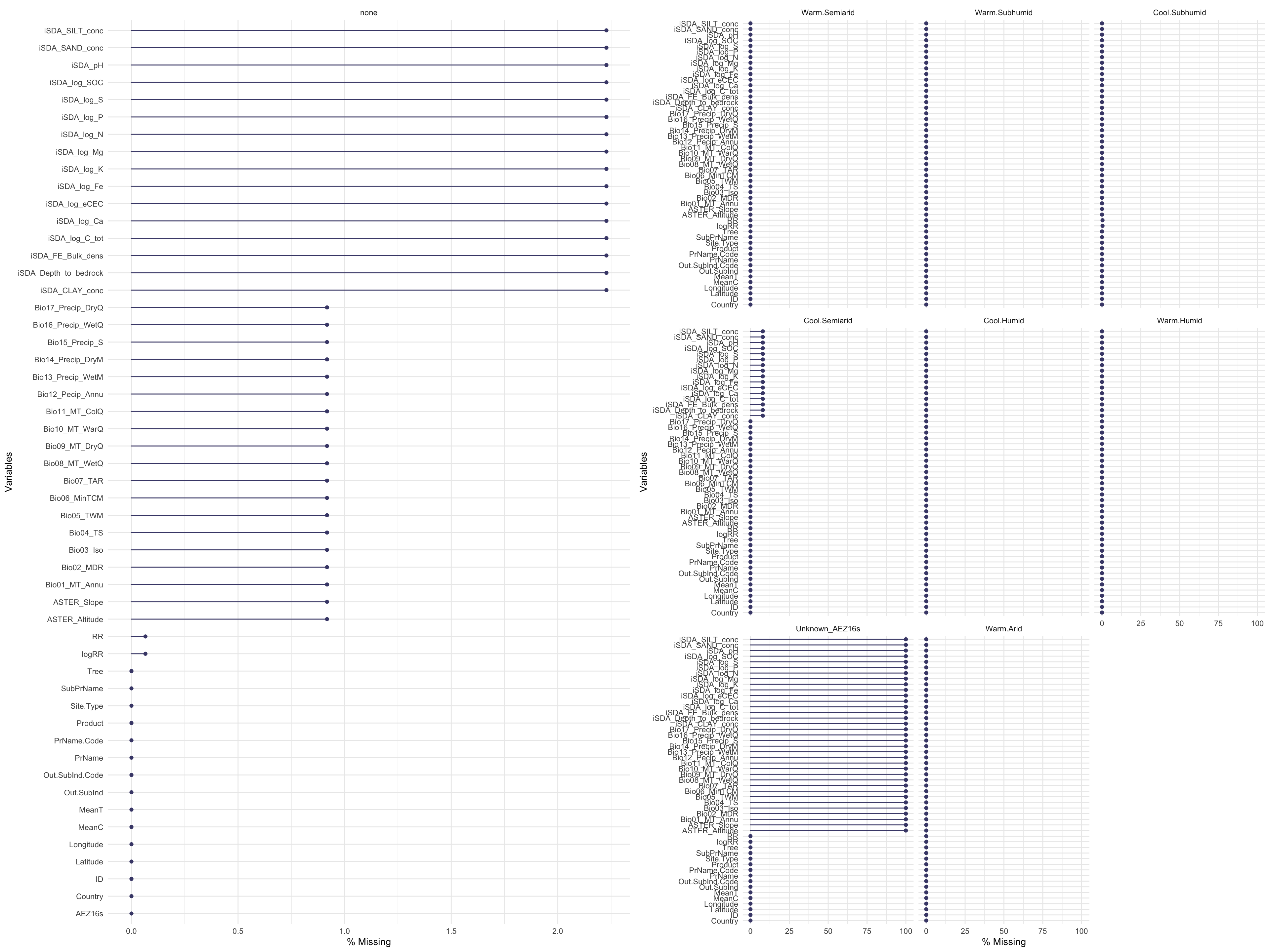
(#fig:Visually assess where we have missing data)Visually assess missing data
Show code
# Warning: It is deprecated to specify `guide = FALSE` to remove a guide. Please use `guide = "none"` instead.
We see that most of data is quite complete however there are some spatially explicit patters for iSDA and WorldClim (BioClim) data. The variable/feature “Tree (species)” is the feature where most data is missing, yet it is only around 20 % of this data we do not have in our agroforestry data. In the faceted plot (by: agroecological zone), we see that there is a great deal of overlap between where we have missing quantitative data, from either iSDA or WorldClim and the missing qualitative information on agroecological zone - again highlighting that some areas/ERA observations are from areas outside the boundary of the co-variables data have been sourced.
Lets look accros the site types (farm, research station and survey) whether we see any differences in missingness of data. To do this we are using the geom_miss_point() function from the naniar package. We are going to plot a random iSDA feature agains a random BioClim feature - as we now know that if there are missing data from one iSDA (or BioClim) feature it is missing in all the features deriving from the respected data source.
agrofor.biophys.selected.features <- readRDS(file = here::here("TidyMod_OUTPUT","agrofor.biophys.selected.features.RDS"))
miss.check.site <-
ggplot(data = agrofor.biophys.selected.features,
aes(x = Bio09_MT_DryQ,
y = iSDA_CLAY_conc)) +
naniar::geom_miss_point() +
facet_wrap(~Site.Type, ncol = 2, scales = "free_x") +
coord_cartesian(ylim = c(-1,60)) +
theme(legend.position = "bottom")
miss.check.country <-
ggplot(data = agrofor.biophys.selected.features,
aes(x = Bio09_MT_DryQ,
y = iSDA_CLAY_conc)) +
naniar::geom_miss_point() +
facet_wrap(~Country, ncol = 2, scales = "free_x") +
coord_cartesian(ylim = c(-1,60)) +
theme(legend.position = "bottom")
Show code
miss.check.site
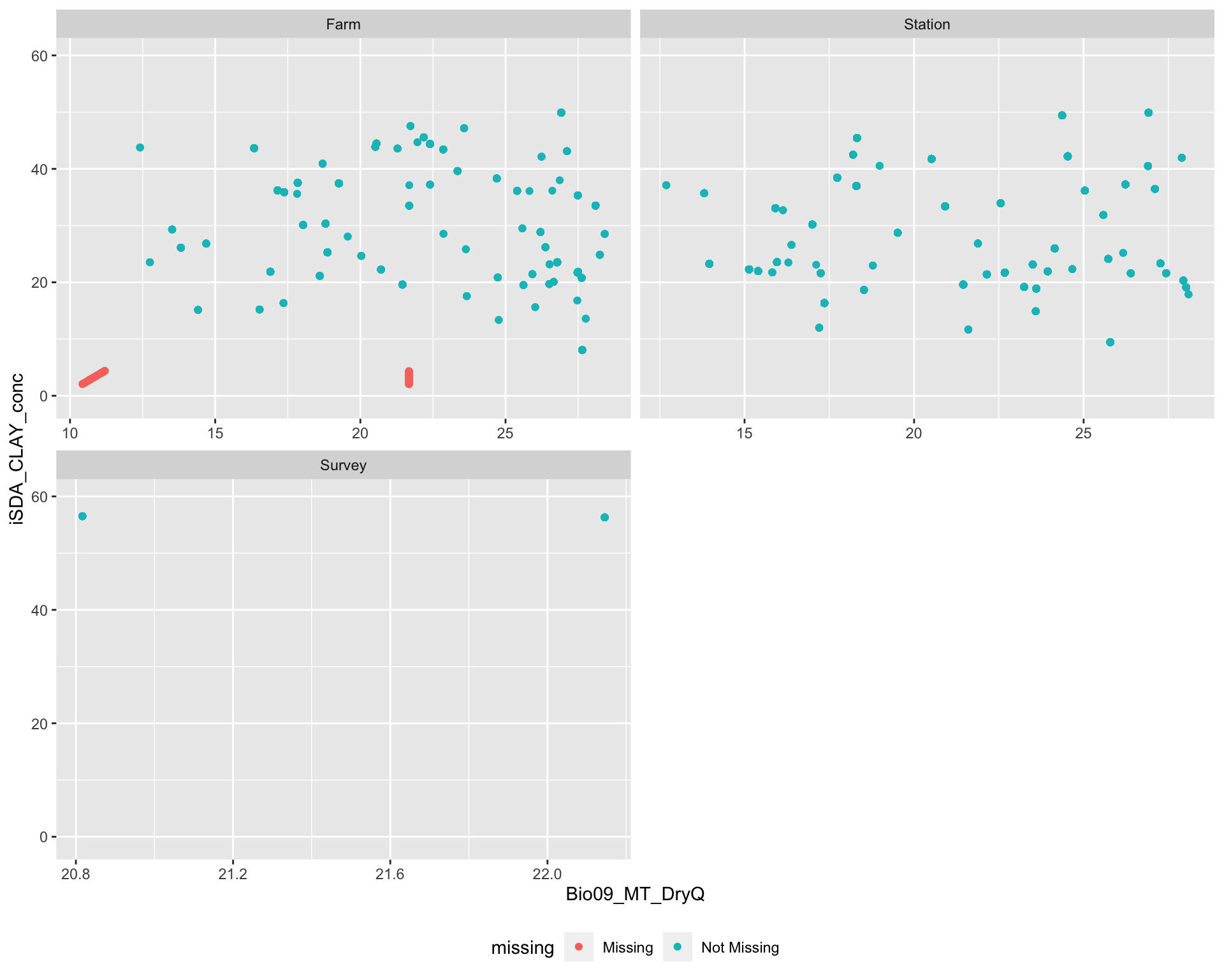
(#fig:Plotting differences in missing data distribution accross site types)Missing data accross site type
..and what about Countries? Do we see differences in the distribution of missing data across Countries?
Show code
miss.check.country
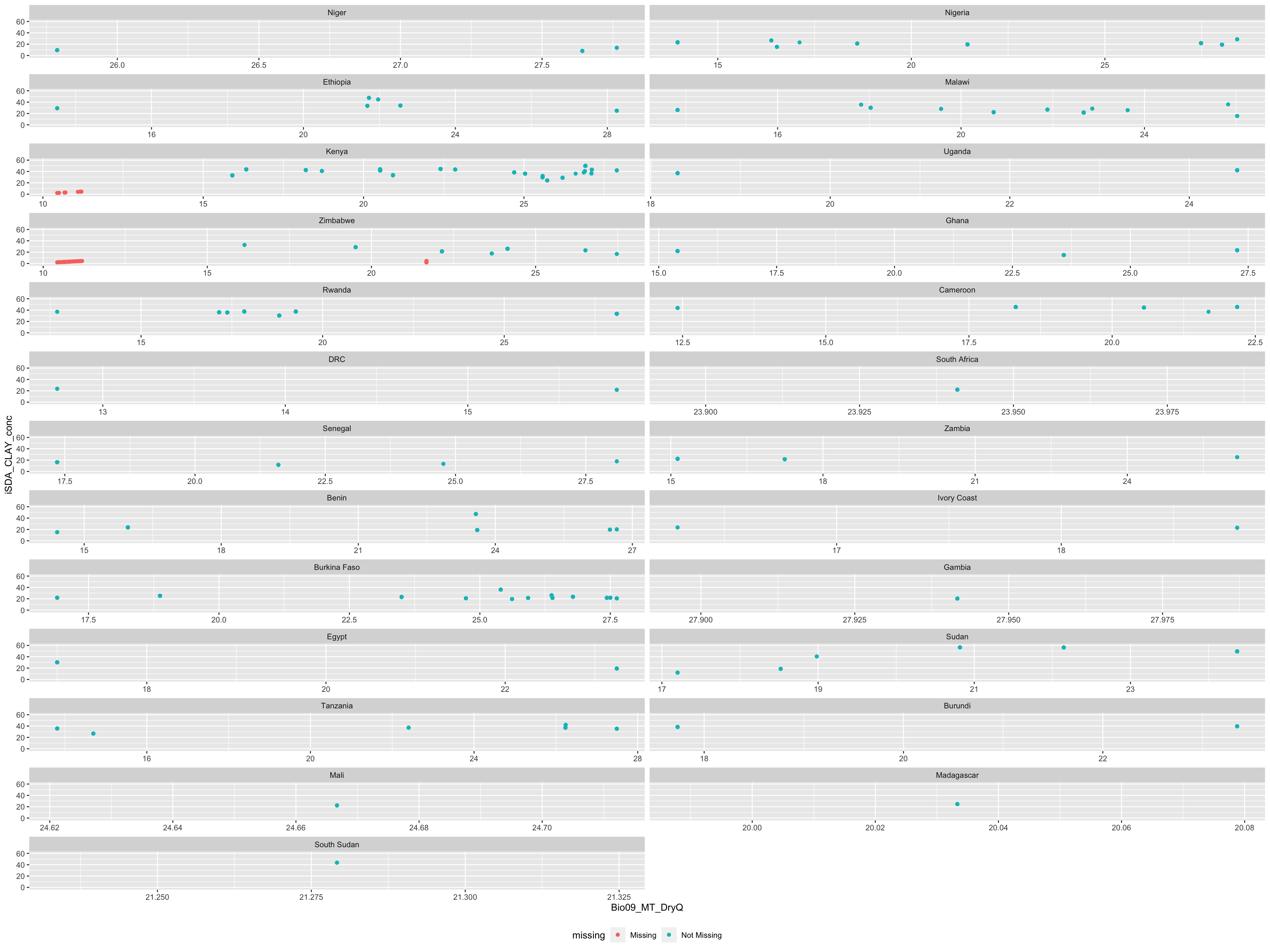
(#fig:Plotting differences in missing data distribution accross contries)Missing data accross Countries
We see that missing data is present only from research sites on farms. We can use the bind_shadow() and nabular() functions from naniar to keep better track of the missing values in our agroforestry data. We also see that Kenya and Zimbabwe are the two major \(sources\) of missing data. This is strange as they are not located outside the countinent.
If we use the nabular table format it helps you manage where missing values are in the dataset and makes it easy to do visualisations where when we split by missingness. Lets look at the missing data overlap between the two co-variables “Bio09_MT_DryQ” and “iSDA_CLAY_conc,” and then visualise a density plot.
Show code
agrofor.biophys.modelling.data.nabular <- naniar::nabular(agrofor.biophys.selected.features)
rmarkdown::paged_table(agrofor.biophys.modelling.data.nabular)
Using the naniar function called bind_shadow() we can generate a visual showing the areas of our agroforestry data where we have missing data. Lets make such a shaddow plot:
Show code
agrofor.biophys.modelling.data.numeric <- readRDS(file = here::here("TidyMod_OUTPUT", "agrofor.biophys.modelling.data.numeric.RDS"))
agrofor.biophys.modelling.data.numeric.shadow <- naniar::bind_shadow(agrofor.biophys.modelling.data.numeric)
# Bio01_MT_Annu
agrofor.biophys.shadow.bind.plot.Bio01 <- agrofor.biophys.modelling.data.numeric.shadow %>%
ggplot(aes(x = logRR,
fill = Bio01_MT_Annu_NA)) +
geom_density(col = "gray", alpha = 0.5, size = 1) +
scale_fill_manual(aesthetics = "fill", values = c("#A2AC8A", "#FED82F")) +
theme_lucid(legend.title.size = 0) +
labs(subtitle = "BIO.01 - Mean annual temperature")
# Bio02_MDR
agrofor.biophys.shadow.bind.plot.Bio02 <- agrofor.biophys.modelling.data.numeric.shadow %>%
ggplot(aes(x = logRR,
fill = Bio02_MDR_NA)) +
geom_density(col = "gray", alpha = 0.5, size = 1) +
scale_fill_manual(aesthetics = "fill", values = c("#A2AC8A", "#FED82F")) +
theme_lucid(legend.title.size = 0) +
labs(subtitle = "BIO.02 - Mean diurnal range")
# Bio03_Iso
agrofor.biophys.shadow.bind.plot.Bio03 <- agrofor.biophys.modelling.data.numeric.shadow %>%
ggplot(aes(x = logRR,
fill = Bio03_Iso_NA)) +
geom_density(col = "gray", alpha = 0.5, size = 1) +
scale_fill_manual(aesthetics = "fill", values = c("#A2AC8A", "#FED82F")) +
theme_lucid(legend.title.size = 0) +
labs(subtitle = "BIO.03 - Isothermality")
# Bio07_TAR
agrofor.biophys.shadow.bind.plot.Bio07 <- agrofor.biophys.modelling.data.numeric.shadow %>%
ggplot(aes(x = logRR,
fill = Bio07_TAR_NA)) +
geom_density(col = "gray", alpha = 0.5, size = 1) +
scale_fill_manual(aesthetics = "fill", values = c("#A2AC8A", "#FED82F")) +
theme_lucid(legend.title.size = 0) +
labs(subtitle = "BIO.07 - Temperature annual range")
# Bio12_Pecip_Annu
agrofor.biophys.shadow.bind.plot.Bio12 <- agrofor.biophys.modelling.data.numeric.shadow %>%
ggplot(aes(x = logRR,
fill = Bio12_Pecip_Annu_NA)) +
geom_density(col = "gray", alpha = 0.5, size = 1) +
scale_fill_manual(aesthetics = "fill", values = c("#A2AC8A", "#FED82F")) +
theme_lucid(legend.title.size = 0) +
labs(subtitle = "BIO.12 - Annual precipitation")
# iSDA_SAND_conc
agrofor.biophys.shadow.bind.plot.sand <- agrofor.biophys.modelling.data.numeric.shadow %>%
ggplot(aes(x = logRR,
fill = iSDA_SAND_conc_NA)) +
geom_density(col = "gray", alpha = 0.5, size = 1) +
scale_fill_manual(aesthetics = "fill", values = c("#A2AC8A", "#FED82F")) +
theme_lucid(legend.title.size = 0) +
labs(subtitle = "iSDA - Sand concentration")
# iSDA_log_C_tot
agrofor.biophys.shadow.bind.plot.totcarbon <- agrofor.biophys.modelling.data.numeric.shadow %>%
ggplot(aes(x = logRR,
fill = iSDA_log_C_tot_NA)) +
geom_density(col = "gray", alpha = 0.5, size = 1) +
scale_fill_manual(aesthetics = "fill", values = c("#A2AC8A", "#FED82F")) +
theme_lucid(legend.title.size = 0) +
labs(subtitle = "iSDA - total carbon")
# iSDA_pH
agrofor.biophys.shadow.bind.plot.pH <- agrofor.biophys.modelling.data.numeric.shadow %>%
ggplot(aes(x = logRR,
fill = iSDA_pH_NA)) +
geom_density(col = "gray", alpha = 0.5, size = 1) +
scale_fill_manual(aesthetics = "fill", values = c("#A2AC8A", "#FED82F")) +
theme_lucid(legend.title.size = 0) +
labs(subtitle = "iSDA - pH")
# iSDA_log_N
agrofor.biophys.shadow.bind.plot.N <- agrofor.biophys.modelling.data.numeric.shadow %>%
ggplot(aes(x = logRR,
fill = iSDA_log_N_NA)) +
geom_density(col = "gray", alpha = 0.5, size = 1) +
scale_fill_manual(aesthetics = "fill", values = c("#A2AC8A", "#FED82F")) +
theme_lucid(legend.title.size = 0) +
labs(subtitle = "iSDA - Nitrogen")
# ASTER_Slope
agrofor.biophys.shadow.bind.plot.slope <- agrofor.biophys.modelling.data.numeric.shadow %>%
ggplot(aes(x = logRR,
fill = ASTER_Slope_NA)) +
geom_density(col = "gray", alpha = 0.5, size = 1) +
scale_fill_manual(aesthetics = "fill", values = c("#A2AC8A", "#FED82F")) +
theme_lucid(legend.title.size = 0) +
labs(subtitle = "ASTER - Slope")
# Extract a legend theme from the yplot that is laid out horizontally
agrofor.biophys.shadow.legend <- get_legend(agrofor.biophys.shadow.bind.plot.Bio01 +
guides(color = guide_legend(nrow = 1)) +
theme_lucid(legend.position = "bottom", legend.title.size = 0))
# Cleaning the yplot for any style or theme
agrofor.biophys.shadow.bind.plot.Bio01 <- agrofor.biophys.shadow.bind.plot.Bio01 + clean_theme() + rremove("legend")
agrofor.biophys.shadow.bind.plot.Bio02 <- agrofor.biophys.shadow.bind.plot.Bio02 + clean_theme() + rremove("legend")
agrofor.biophys.shadow.bind.plot.Bio03 <- agrofor.biophys.shadow.bind.plot.Bio03 + clean_theme() + rremove("legend")
agrofor.biophys.shadow.bind.plot.Bio07 <- agrofor.biophys.shadow.bind.plot.Bio07 + clean_theme() + rremove("legend")
agrofor.biophys.shadow.bind.plot.Bio12 <- agrofor.biophys.shadow.bind.plot.Bio12 + clean_theme() + rremove("legend")
agrofor.biophys.shadow.bind.plot.sand <- agrofor.biophys.shadow.bind.plot.sand + clean_theme() + rremove("legend")
agrofor.biophys.shadow.bind.plot.pH <- agrofor.biophys.shadow.bind.plot.pH + clean_theme() + rremove("legend")
agrofor.biophys.shadow.bind.plot.N <- agrofor.biophys.shadow.bind.plot.N + clean_theme() + rremove("legend")
agrofor.biophys.shadow.bind.plot.totcarbon <- agrofor.biophys.shadow.bind.plot.totcarbon + clean_theme() + rremove("legend")
agrofor.biophys.shadow.bind.plot.slope <- agrofor.biophys.shadow.bind.plot.slope + clean_theme() + rremove("legend")
# Creating the title
# add margin on the left of the drawing canvas,
# so title is aligned with left edge of first plot
agrofor.biophys.shadow.title <- ggdraw() +
draw_label(
"Combined shaddow density plot of missing value distribution of selected biophysical predictors vs. logRR",
fontface = 'bold',
x = 0,
hjust = 0,
size = 20) +
theme(plot.margin = margin(0, 0, 0, 7))
# Warning: Removed 15 rows containing non-finite values (stat_density).
Lets combine these in a cowplot
Show code
# Arranging the plots and using cowplot::plot_grid() to plot the three plots together
combined.agrofor.biophys.shadow <- cowplot::plot_grid(
agrofor.biophys.shadow.title,
NULL,
NULL,
#########
agrofor.biophys.shadow.bind.plot.Bio01,
agrofor.biophys.shadow.bind.plot.Bio02,
agrofor.biophys.shadow.bind.plot.Bio03,
agrofor.biophys.shadow.bind.plot.Bio07,
agrofor.biophys.shadow.bind.plot.Bio12,
agrofor.biophys.shadow.bind.plot.sand,
agrofor.biophys.shadow.bind.plot.pH,
agrofor.biophys.shadow.bind.plot.N,
agrofor.biophys.shadow.bind.plot.totcarbon,
agrofor.biophys.shadow.bind.plot.slope,
#########
agrofor.biophys.shadow.legend,
#########
ncol = 3, nrow = 5, align = "hv",
rel_widths = c(1, 1, 1),
rel_heights = c(2, 2, 2, 2))
combined.agrofor.biophys.shadow
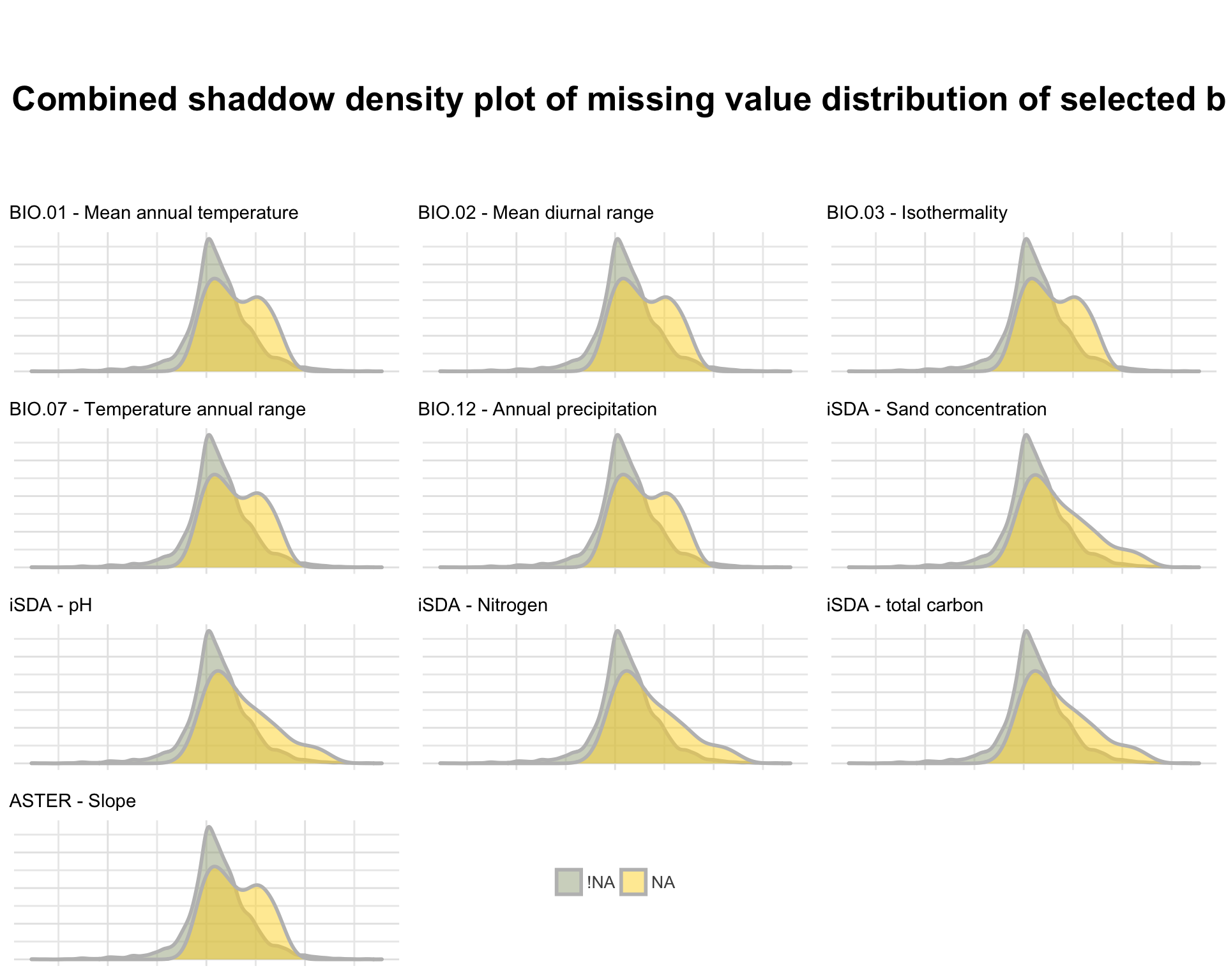
Figure 1: Shaddow plot of selected biophysical predictor features
Show code
# Warning: Removed 15 rows containing non-finite values (stat_density).
# Warning: Graphs cannot be vertically aligned unless the axis parameter is set. Placing graphs unaligned.
# Warning: Graphs cannot be horizontally aligned unless the axis parameter is set. Placing graphs unaligned.
We see again that there is a spatial relation between the missingness of our data, as the pattern is similar for the features extracted from the same data sources. Therefore there must be some areas where we have no biophysical information. This is perhaps because the biophysical co-variables are extracted from a fixed boundary of the African continent and islands such as Capo Verde is situated outside the continent.
Density distributions of features
Until this point we have identified and familiarised ourself with the missing data. We can now make a clean numeric dataset in which we remove all NA observations. This will be helpful for the further process of EDA. For a more aesthetic experience we are also making a custom colour range of 35 colours that we can use to plot our 35 predictors with.
expl.agfor.data.no.na <- agrofor.biophys.modelling.data.numeric %>%
rationalize() %>%
drop_na()
dim(agrofor.biophys.modelling.data.numeric) # <- before removing NAs
# [1] 4578 37
dim(expl.agfor.data.no.na) # <- after removing NAs
# [1] 4461 37
# Colour range with 35 levels
nb.cols.35 <- 35
era.af.colors.35 <- colorRampPalette(brewer.pal(8, "Set2"))(nb.cols.35)
Show code
$page_1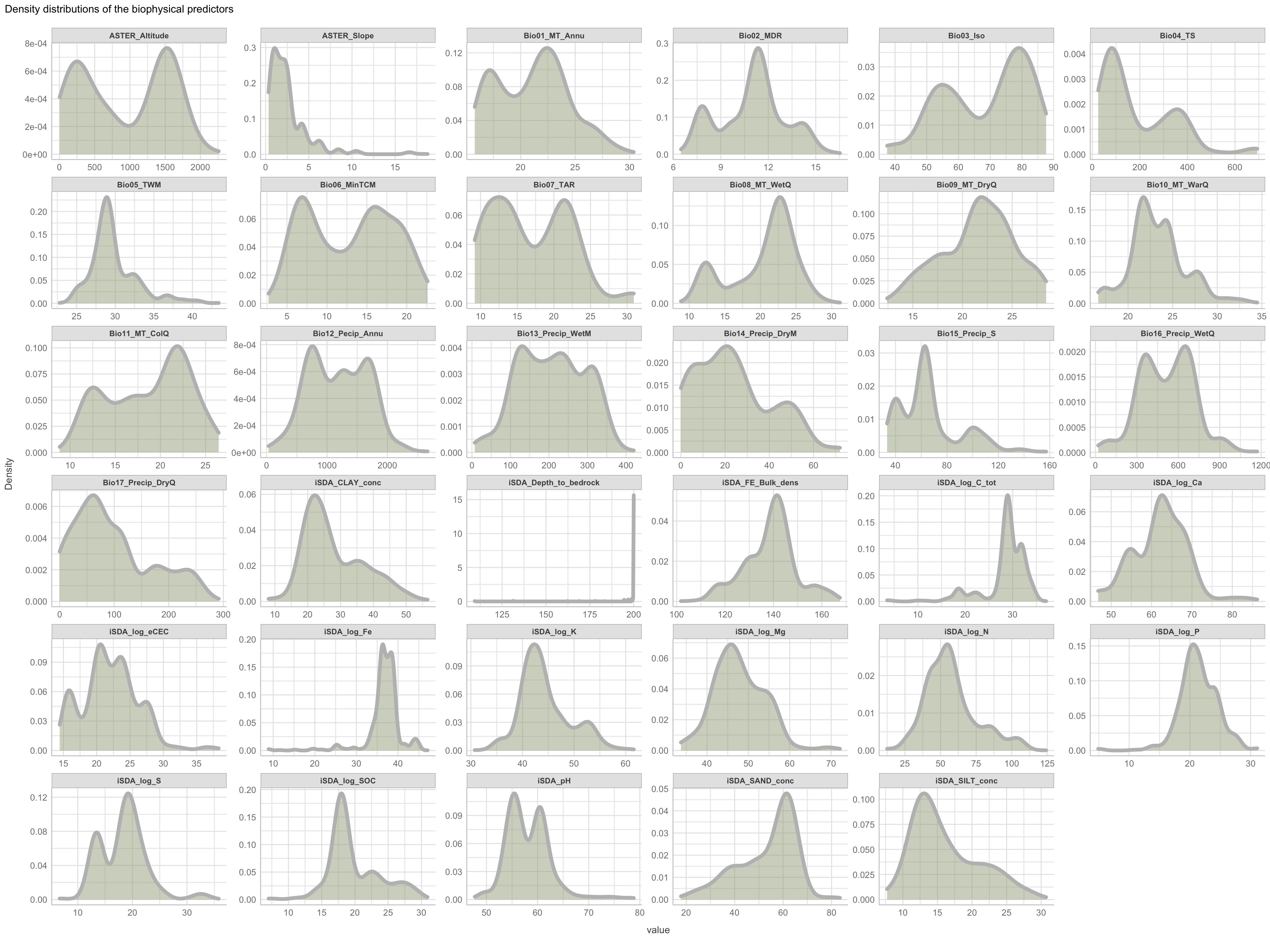
Figure 2: Density distributions of biophysical predictors
Not surprising we see a lot of variation in the density distribution for our biophysical predictors. Some of them shows a multimodal distribution patterns, e.g. altitude and Bio06 the minimum temperature of coldest month, Bio03 the Isothermality and iSDA pH shows a bimodal density distribution pattern, while others, such as Bio05 maximum temperature of warmest month, iSDA Iron concentrations and iSDA total carbon are skewed to the left, right and right, respectfully. Others, like Bio09 mean temperature of driest quarter and iSDA phosphorus concentrations seems to be having a good similarity of a normal distribution. This and other observations gives us a good understanding about the predictors. One take-away massage would be that we clearly need some sort of normalisation and centralisation of the predictors prior to our machine learning exercise in order to get good performance.
Show code
expl.agfor.dens.outcome <- expl.agfor.data.no.na %>%
dplyr::select(c("RR", "logRR")) %>%
plot_density(ggtheme = theme_lucid(),
geom_density_args = list("fill" = "#FED82F", "col" = "gray", "alpha" = 0.5, "size" = 2, "adjust" = 0.5),
ncol = 2, nrow = 1,
parallel = FALSE,
title = "Density distributions of the outcome logRR or RR"
)
Show code
$page_1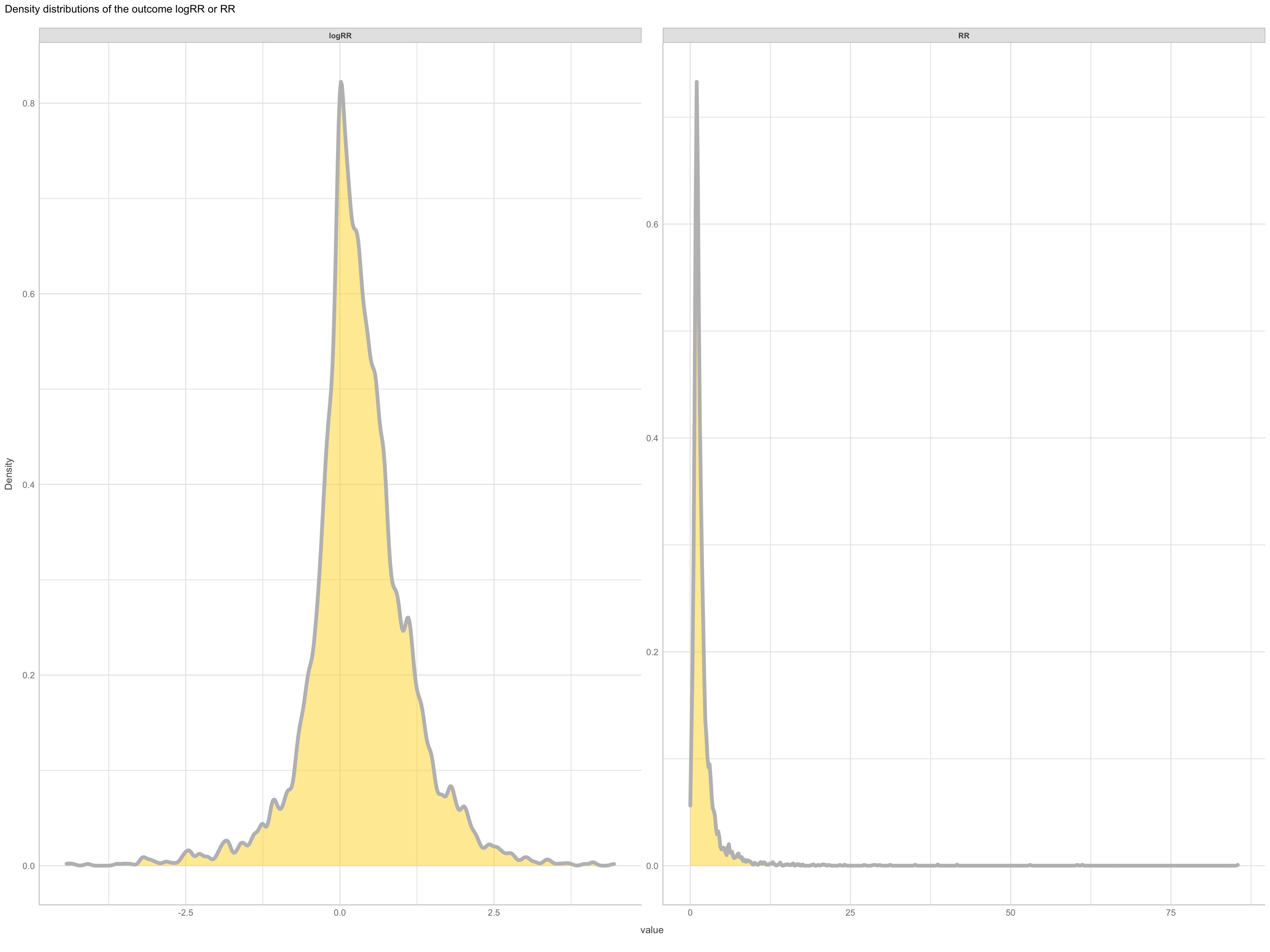
(#fig:logRR density distrubution)Density distributions logRR
It is not only the destribution of predictors that matter when doing machine learning modelling, and in order to get a good performance we also need to check for normality in our outcome feature as they will be difficult for the algorithm to predict if we have too abnormall patterns. So lets view the density distribution for our outcome feature(s) logRR and RR.
This clearly demonstrate that the log transformed RR is a much better outcome feature, compared to the raw RR. We might want to exclude extreme values from our logRR on both the positive and negative tail of the distribution. We might do this using the extreme outlier removal approach already used in the ERAAnalyze function, where response ratios above or below 3∗IQR (interquartile range) are removed.
is_outlier <- function(x) {
return(x < quantile(x, 0.25) - 3 * IQR(x) | x > quantile(x, 0.75) + 3 * IQR(x))
}
expl.agfor.data.no.na.logRR.outlier <- expl.agfor.data.no.na %>%
mutate(ERA_Agroforestry = 1) %>%
group_by(ERA_Agroforestry) %>%
mutate(logRR.outlier = ifelse(is_outlier(logRR), logRR, as.numeric(NA)))
# SAVING DATA
saveRDS(expl.agfor.data.no.na.logRR.outlier, here::here("TidyMod_OUTPUT", "expl.agfor.data.no.na.logRR.outlier.RDS"))
Show code
expl.agfor.data.no.na.logRR.outlier <- readRDS(here::here("TidyMod_OUTPUT", "expl.agfor.data.no.na.logRR.outlier.RDS"))
rmarkdown::paged_table(expl.agfor.data.no.na.logRR.outlier %>% count(logRR.outlier, sort = TRUE))
Based on the extreme outliers removal method we have 40 outliers with 28 of them being < 0 and 12 being > 0. Lets assess these outliers visually by making a nice violin and box plot of the outcome variable logRR using ggplot2 with the ggbeeswarm package. We will include the outliers indicated in red within the 3 * QR limit.
Show code
ggplot_box_legend <- function(family = "serif"){
# Create data to use in the boxplot legend:
set.seed(100)
sample_df <- data.frame(parameter = "test",
values = sample(500))
# Extend the top whisker a bit:
sample_df$values[1:100] <- 701:800
# Make sure there's only 1 lower outlier:
sample_df$values[1] <- -350
# Function to calculate important values:
ggplot2_boxplot <- function(x){
quartiles <- as.numeric(quantile(x,
probs = c(0.25, 0.5, 0.75)))
names(quartiles) <- c("25th percentile",
"50th percentile\n(median)",
"75th percentile")
IQR <- diff(quartiles[c(1,3)])
upper_whisker <- max(x[x < (quartiles[3] + 1.5 * IQR)])
lower_whisker <- min(x[x > (quartiles[1] - 1.5 * IQR)])
upper_dots <- x[x > (quartiles[3] + 1.5*IQR)]
lower_dots <- x[x < (quartiles[1] - 1.5*IQR)]
return(list("quartiles" = quartiles,
"25th percentile" = as.numeric(quartiles[1]),
"50th percentile\n(median)" = as.numeric(quartiles[2]),
"75th percentile" = as.numeric(quartiles[3]),
"IQR" = IQR,
"upper_whisker" = upper_whisker,
"lower_whisker" = lower_whisker,
"upper_dots" = upper_dots,
"lower_dots" = lower_dots))
}
# Get those values:
ggplot_output <- ggplot2_boxplot(sample_df$values)
# Lots of text in the legend, make it smaller and consistent font:
update_geom_defaults("text",
list(size = 3,
hjust = 0,
family = family))
# Labels don't inherit text:
update_geom_defaults("label",
list(size = 3,
hjust = 0,
family = family))
# Create the legend:
# The main elements of the plot (the boxplot, error bars, and count)
# are the easy part.
# The text describing each of those takes a lot of fiddling to
# get the location and style just right:
explain_plot <- ggplot() +
geom_violin(data = sample_df,
aes(x = parameter, y = values),
alpha = 0.5,
size = 4,
fill = "#FED82F",
colour = "white",
width = 0.3) +
geom_boxplot(data = sample_df,
aes(x = parameter, y = values),
fill = "white",
col = "black",
notch = TRUE,
outlier.size = 0.3,
lwd = 1,
alpha = 0.5,
outlier.colour = "red",
outlier.fill = "black",
show.legend = F,
outlier.shape = 10) +
stat_boxplot(data = sample_df,
aes(x = parameter, y = values),
alpha = 0.3,
size = 1,
geom = "errorbar",
colour = "black",
linetype = 1,
width = 0.3) + #whiskers+
geom_text(aes(x = 1, y = 950, label = ""), hjust = 0.5) +
geom_text(aes(x = 1.17, y = 950,
label = ""),
fontface = "bold", vjust = 0.4) +
theme_minimal(base_size = 5, base_family = family) +
geom_segment(aes(x = 2.3, xend = 2.3,
y = ggplot_output[["25th percentile"]],
yend = ggplot_output[["75th percentile"]])) +
geom_segment(aes(x = 1.2, xend = 2.3,
y = ggplot_output[["25th percentile"]],
yend = ggplot_output[["25th percentile"]])) +
geom_segment(aes(x = 1.2, xend = 2.3,
y = ggplot_output[["75th percentile"]],
yend = ggplot_output[["75th percentile"]])) +
geom_text(aes(x = 2.4, y = ggplot_output[["50th percentile\n(median)"]]),
label = "Interquartile\nrange", fontface = "bold",
vjust = 0.4) +
geom_text(aes(x = c(1.17,1.17),
y = c(ggplot_output[["upper_whisker"]],
ggplot_output[["lower_whisker"]]),
label = c("Largest value within 3 times\ninterquartile range above\n75th percentile",
"Smallest value within 3 times\ninterquartile range below\n25th percentile")),
fontface = "bold", vjust = 0.9) +
geom_text(aes(x = c(1.17),
y = ggplot_output[["lower_dots"]],
label = "Outside value"),
vjust = 0.5, fontface = "bold") +
geom_text(aes(x = c(1.9),
y = ggplot_output[["lower_dots"]],
label = "-Value is > and/or < 3 times"),
vjust = 0.5) +
geom_text(aes(x = 1.17,
y = ggplot_output[["lower_dots"]],
label = "the interquartile range\nbeyond either end of the box"),
vjust = 1.5) +
geom_label(aes(x = 1.17, y = ggplot_output[["quartiles"]],
label = names(ggplot_output[["quartiles"]])),
vjust = c(0.4,0.85,0.4),
fill = "white", label.size = 0) +
ylab("") + xlab("") +
theme(axis.text = element_blank(),
axis.ticks = element_blank(),
panel.grid = element_blank(),
aspect.ratio = 4/3,
plot.title = element_text(hjust = 0.5, size = 10)) +
coord_cartesian(xlim = c(1.4,3.1), ylim = c(-600, 900)) +
labs(title = "EXPLANATION")
return(explain_plot)
}
Creating logRR outliers plot
Show code
legend_plot <- ggplot_box_legend()
logRR.outlier.plot <-
ggplot(data = expl.agfor.data.no.na.logRR.outlier, aes(y = logRR, x = "ERA_Agroforestry")) +
scale_fill_viridis_d( option = "D") +
geom_violin(alpha = 0.5, position = position_dodge(width = 1), size = 1, fill = "#FED82F", colour = "white") +
geom_boxplot(notch = TRUE, outlier.size = 0.3, color = "black", lwd = 1, alpha = 0.5, outlier.colour = "red",
outlier.fill = "black", show.legend = F, outlier.shape = 10) +
scale_y_continuous(breaks =seq(-5, 5, 0.5), limit = c(-6, 6)) +
stat_boxplot(geom ='errorbar', width = 0.15, coef = 3) +
geom_text(aes(label = logRR.outlier), na.rm = TRUE, hjust = -0.3) +
# geom_point( shape = 21,size=2, position = position_jitterdodge(), color="black",alpha=1)+
ggbeeswarm::geom_quasirandom(shape = 21, size = 1, dodge.width = 0.5, color = "black", alpha = 0.3, show.legend = F) +
theme_minimal() +
ylab(c("logRR")) +
xlab("All ERA Agroforestry Data") +
theme(#panel.border = element_rect(colour = "black", fill=NA, size=2),
axis.line = element_line(colour = "black" , size = 1),
axis.ticks = element_line(size = 1, color = "black"),
axis.text = element_text(color = "black"),
axis.ticks.length = unit(0.5, "cm"),
legend.position = "none") +
font("xylab", size = 15) +
font("xy", size = 15) +
font("xy.text", size = 15) +
font("legend.text", size = 15) +
guides(fill = guide_legend(override.aes = list(alpha = 0.3, color = "black")))
logRR.outlier.plot.title <- ggdraw() +
draw_label(
"ERA agroforestry logRR violin and boxplot with outliers",
fontface = 'bold',
x = 0,
hjust = 0,
size = 20) +
theme(plot.margin = margin(0, 0, 0, 7))
Show code
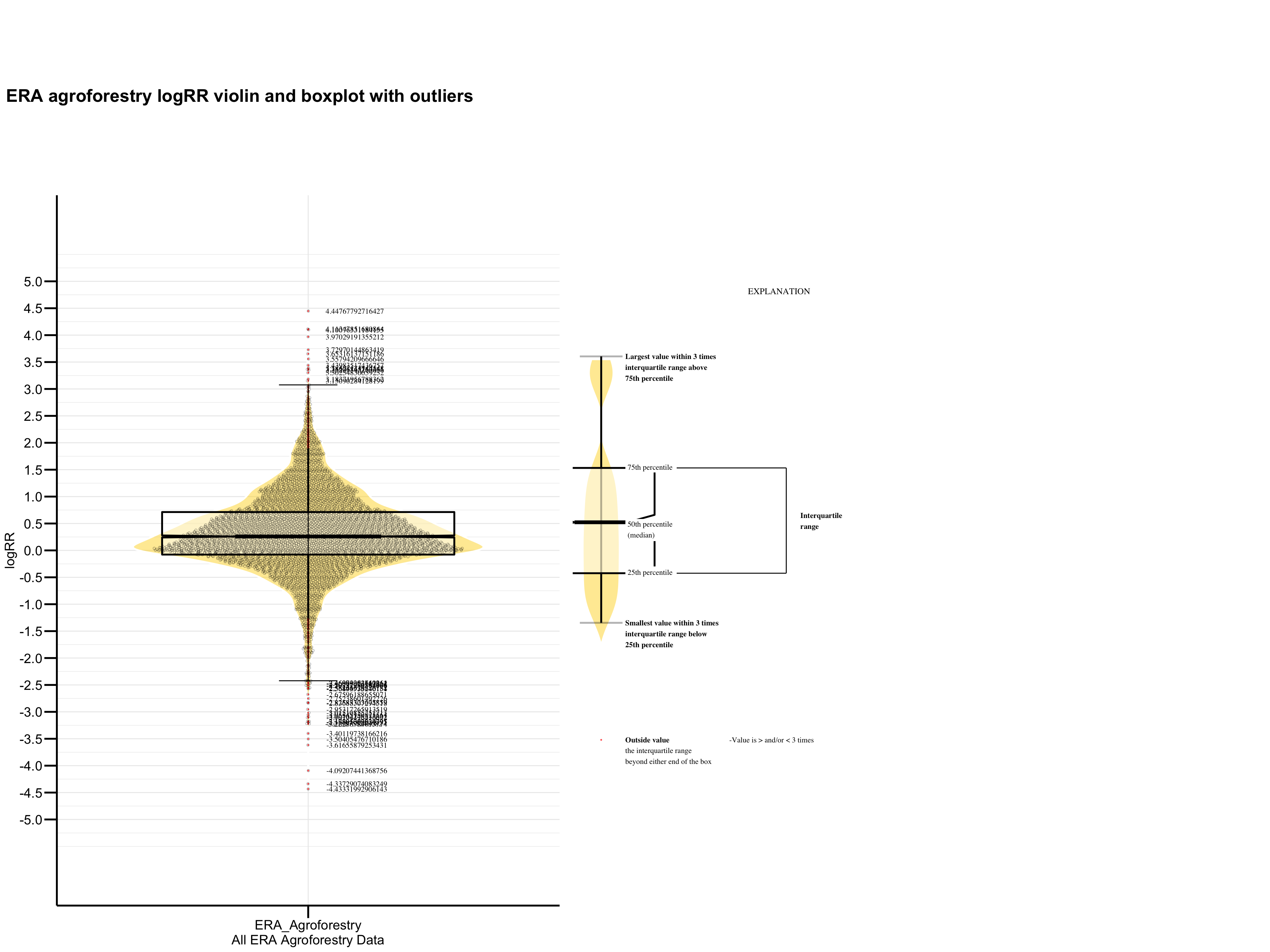
Figure 3: logRR outliers plot
We see that there are some logRR observation we would have to remove in order for our machine learning models to perform well!
Histograms of biophysical predictor features
Lets now look at the histograms of our biophysical predictors. This is slightly similar to the density plots, but with the histograms we are able to see how the data is distributed in bins of 30 observations each. We are using the plot_histogram() from the DataExplorer package. The way we are going to plot the histogram requires a custom colour specification that has more than 1000 color objects specified.
Generating custom colour object with 1050 colours
Show code
# 1050 levels of 35 colours
explor.cols.group.35_1050 <- c("#66C2A5", "#66C2A5", "#66C2A5", "#66C2A5", "#66C2A5",
"#66C2A5", "#66C2A5", "#66C2A5", "#66C2A5", "#66C2A5",
"#66C2A5", "#66C2A5", "#66C2A5", "#66C2A5", "#66C2A5",
"#66C2A5", "#66C2A5", "#66C2A5", "#66C2A5", "#66C2A5",
"#66C2A5", "#66C2A5", "#66C2A5", "#66C2A5", "#66C2A5",
"#66C2A5", "#66C2A5", "#66C2A5", "#66C2A5", "#66C2A5",
"#84B797", "#84B797", "#84B797", "#84B797", "#84B797",
"#84B797", "#84B797", "#84B797", "#84B797", "#84B797",
"#84B797", "#84B797", "#84B797", "#84B797", "#84B797",
"#84B797", "#84B797", "#84B797", "#84B797", "#84B797",
"#84B797", "#84B797", "#84B797", "#84B797", "#84B797",
"#84B797", "#84B797", "#84B797", "#84B797", "#84B797",
"#A2AC8A", "#A2AC8A", "#A2AC8A", "#A2AC8A", "#A2AC8A",
"#A2AC8A", "#A2AC8A", "#A2AC8A", "#A2AC8A", "#A2AC8A",
"#A2AC8A", "#A2AC8A", "#A2AC8A", "#A2AC8A", "#A2AC8A",
"#A2AC8A", "#A2AC8A", "#A2AC8A", "#A2AC8A", "#A2AC8A",
"#A2AC8A", "#A2AC8A", "#A2AC8A", "#A2AC8A", "#A2AC8A",
"#A2AC8A", "#A2AC8A", "#A2AC8A", "#A2AC8A", "#A2AC8A",
"#C0A27C", "#C0A27C", "#C0A27C", "#C0A27C", "#C0A27C",
"#C0A27C", "#C0A27C", "#C0A27C", "#C0A27C", "#C0A27C",
"#C0A27C", "#C0A27C", "#C0A27C", "#C0A27C", "#C0A27C",
"#C0A27C", "#C0A27C", "#C0A27C", "#C0A27C", "#C0A27C",
"#C0A27C", "#C0A27C", "#C0A27C", "#C0A27C", "#C0A27C",
"#C0A27C", "#C0A27C", "#C0A27C", "#C0A27C", "#C0A27C",
"#DE976F", "#DE976F", "#DE976F", "#DE976F", "#DE976F",
"#DE976F", "#DE976F", "#DE976F", "#DE976F", "#DE976F",
"#DE976F", "#DE976F", "#DE976F", "#DE976F", "#DE976F",
"#DE976F", "#DE976F", "#DE976F", "#DE976F", "#DE976F",
"#DE976F", "#DE976F", "#DE976F", "#DE976F", "#DE976F",
"#DE976F", "#DE976F", "#DE976F", "#DE976F", "#DE976F",
"#FC8D62", "#FC8D62", "#FC8D62", "#FC8D62", "#FC8D62",
"#FC8D62", "#FC8D62", "#FC8D62", "#FC8D62", "#FC8D62",
"#FC8D62", "#FC8D62", "#FC8D62", "#FC8D62", "#FC8D62",
"#FC8D62", "#FC8D62", "#FC8D62", "#FC8D62", "#FC8D62",
"#FC8D62", "#FC8D62", "#FC8D62", "#FC8D62", "#FC8D62",
"#FC8D62", "#FC8D62", "#FC8D62", "#FC8D62", "#FC8D62",
"#E59077", "#E59077", "#E59077", "#E59077", "#E59077",
"#E59077", "#E59077", "#E59077", "#E59077", "#E59077",
"#E59077", "#E59077", "#E59077", "#E59077", "#E59077",
"#E59077", "#E59077", "#E59077", "#E59077", "#E59077",
"#E59077", "#E59077", "#E59077", "#E59077", "#E59077",
"#E59077", "#E59077", "#E59077", "#E59077", "#E59077",
"#CF948C", "#CF948C", "#CF948C", "#CF948C", "#CF948C",
"#CF948C", "#CF948C", "#CF948C", "#CF948C", "#CF948C",
"#CF948C", "#CF948C", "#CF948C", "#CF948C", "#CF948C",
"#CF948C", "#CF948C", "#CF948C", "#CF948C", "#CF948C",
"#CF948C", "#CF948C", "#CF948C", "#CF948C", "#CF948C",
"#CF948C", "#CF948C", "#CF948C", "#CF948C", "#CF948C",
"#B998A1", "#B998A1", "#B998A1", "#B998A1", "#B998A1",
"#B998A1", "#B998A1", "#B998A1", "#B998A1", "#B998A1",
"#B998A1", "#B998A1", "#B998A1", "#B998A1", "#B998A1",
"#B998A1", "#B998A1", "#B998A1", "#B998A1", "#B998A1",
"#B998A1", "#B998A1", "#B998A1", "#B998A1", "#B998A1",
"#B998A1", "#B998A1", "#B998A1", "#B998A1", "#B998A1",
"#A39CB5", "#A39CB5", "#A39CB5", "#A39CB5", "#A39CB5",
"#A39CB5", "#A39CB5", "#A39CB5", "#A39CB5", "#A39CB5",
"#A39CB5", "#A39CB5", "#A39CB5", "#A39CB5", "#A39CB5",
"#A39CB5", "#A39CB5", "#A39CB5", "#A39CB5", "#A39CB5",
"#A39CB5", "#A39CB5", "#A39CB5", "#A39CB5", "#A39CB5",
"#A39CB5", "#A39CB5", "#A39CB5", "#A39CB5", "#A39CB5",
"#8DA0CB", "#8DA0CB", "#8DA0CB", "#8DA0CB", "#8DA0CB",
"#8DA0CB", "#8DA0CB", "#8DA0CB", "#8DA0CB", "#8DA0CB",
"#8DA0CB", "#8DA0CB", "#8DA0CB", "#8DA0CB", "#8DA0CB",
"#8DA0CB", "#8DA0CB", "#8DA0CB", "#8DA0CB", "#8DA0CB",
"#8DA0CB", "#8DA0CB", "#8DA0CB", "#8DA0CB", "#8DA0CB",
"#8DA0CB", "#8DA0CB", "#8DA0CB", "#8DA0CB", "#8DA0CB",
"#9F9BC9", "#9F9BC9", "#9F9BC9", "#9F9BC9", "#9F9BC9",
"#9F9BC9", "#9F9BC9", "#9F9BC9", "#9F9BC9", "#9F9BC9",
"#9F9BC9", "#9F9BC9", "#9F9BC9", "#9F9BC9", "#9F9BC9",
"#9F9BC9", "#9F9BC9", "#9F9BC9", "#9F9BC9", "#9F9BC9",
"#9F9BC9", "#9F9BC9", "#9F9BC9", "#9F9BC9", "#9F9BC9",
"#9F9BC9", "#9F9BC9", "#9F9BC9", "#9F9BC9", "#9F9BC9",
"#B197C7", "#B197C7", "#B197C7", "#B197C7", "#B197C7",
"#B197C7", "#B197C7", "#B197C7", "#B197C7", "#B197C7",
"#B197C7", "#B197C7", "#B197C7", "#B197C7", "#B197C7",
"#B197C7", "#B197C7", "#B197C7", "#B197C7", "#B197C7",
"#B197C7", "#B197C7", "#B197C7", "#B197C7", "#B197C7",
"#B197C7", "#B197C7", "#B197C7", "#B197C7", "#B197C7",
"#C392C6", "#C392C6", "#C392C6", "#C392C6", "#C392C6",
"#C392C6", "#C392C6", "#C392C6", "#C392C6", "#C392C6",
"#C392C6", "#C392C6", "#C392C6", "#C392C6", "#C392C6",
"#C392C6", "#C392C6", "#C392C6", "#C392C6", "#C392C6",
"#C392C6", "#C392C6", "#C392C6", "#C392C6", "#C392C6",
"#C392C6", "#C392C6", "#C392C6", "#C392C6", "#C392C6",
"#D48EC4", "#D48EC4", "#D48EC4", "#D48EC4", "#D48EC4",
"#D48EC4", "#D48EC4", "#D48EC4", "#D48EC4", "#D48EC4",
"#D48EC4", "#D48EC4", "#D48EC4", "#D48EC4", "#D48EC4",
"#D48EC4", "#D48EC4", "#D48EC4", "#D48EC4", "#D48EC4",
"#D48EC4", "#D48EC4", "#D48EC4", "#D48EC4", "#D48EC4",
"#D48EC4", "#D48EC4", "#D48EC4", "#D48EC4", "#D48EC4",
"#E78AC3", "#E78AC3", "#E78AC3", "#E78AC3", "#E78AC3",
"#E78AC3", "#E78AC3", "#E78AC3", "#E78AC3", "#E78AC3",
"#E78AC3", "#E78AC3", "#E78AC3", "#E78AC3", "#E78AC3",
"#E78AC3", "#E78AC3", "#E78AC3", "#E78AC3", "#E78AC3",
"#E78AC3", "#E78AC3", "#E78AC3", "#E78AC3", "#E78AC3",
"#E78AC3", "#E78AC3", "#E78AC3", "#E78AC3", "#E78AC3",
"#DA99AC", "#DA99AC", "#DA99AC", "#DA99AC", "#DA99AC",
"#DA99AC", "#DA99AC", "#DA99AC", "#DA99AC", "#DA99AC",
"#DA99AC", "#DA99AC", "#DA99AC", "#DA99AC", "#DA99AC",
"#DA99AC", "#DA99AC", "#DA99AC", "#DA99AC", "#DA99AC",
"#DA99AC", "#DA99AC", "#DA99AC", "#DA99AC", "#DA99AC",
"#DA99AC", "#DA99AC", "#DA99AC", "#DA99AC", "#DA99AC",
"#CDA996", "#CDA996", "#CDA996", "#CDA996", "#CDA996",
"#CDA996", "#CDA996", "#CDA996", "#CDA996", "#CDA996",
"#CDA996", "#CDA996", "#CDA996", "#CDA996", "#CDA996",
"#CDA996", "#CDA996", "#CDA996", "#CDA996", "#CDA996",
"#CDA996", "#CDA996", "#CDA996", "#CDA996", "#CDA996",
"#CDA996", "#CDA996", "#CDA996", "#CDA996", "#CDA996",
"#C0B880", "#C0B880", "#C0B880", "#C0B880", "#C0B880",
"#C0B880", "#C0B880", "#C0B880", "#C0B880", "#C0B880",
"#C0B880", "#C0B880", "#C0B880", "#C0B880", "#C0B880",
"#C0B880", "#C0B880", "#C0B880", "#C0B880", "#C0B880",
"#C0B880", "#C0B880", "#C0B880", "#C0B880", "#C0B880",
"#C0B880", "#C0B880", "#C0B880", "#C0B880", "#C0B880",
"#B3C86A", "#B3C86A", "#B3C86A", "#B3C86A", "#B3C86A",
"#B3C86A", "#B3C86A", "#B3C86A", "#B3C86A", "#B3C86A",
"#B3C86A", "#B3C86A", "#B3C86A", "#B3C86A", "#B3C86A",
"#B3C86A", "#B3C86A", "#B3C86A", "#B3C86A", "#B3C86A",
"#B3C86A", "#B3C86A", "#B3C86A", "#B3C86A", "#B3C86A",
"#B3C86A", "#B3C86A", "#B3C86A", "#B3C86A", "#B3C86A",
"#A6D854", "#A6D854", "#A6D854", "#A6D854", "#A6D854",
"#A6D854", "#A6D854", "#A6D854", "#A6D854", "#A6D854",
"#A6D854", "#A6D854", "#A6D854", "#A6D854", "#A6D854",
"#A6D854", "#A6D854", "#A6D854", "#A6D854", "#A6D854",
"#A6D854", "#A6D854", "#A6D854", "#A6D854", "#A6D854",
"#A6D854", "#A6D854", "#A6D854", "#A6D854", "#A6D854",
"#B7D84C", "#B7D84C", "#B7D84C", "#B7D84C", "#B7D84C",
"#B7D84C", "#B7D84C", "#B7D84C", "#B7D84C", "#B7D84C",
"#B7D84C", "#B7D84C", "#B7D84C", "#B7D84C", "#B7D84C",
"#B7D84C", "#B7D84C", "#B7D84C", "#B7D84C", "#B7D84C",
"#B7D84C", "#B7D84C", "#B7D84C", "#B7D84C", "#B7D84C",
"#B7D84C", "#B7D84C", "#B7D84C", "#B7D84C", "#B7D84C",
"#C9D845", "#C9D845", "#C9D845", "#C9D845", "#C9D845",
"#C9D845", "#C9D845", "#C9D845", "#C9D845", "#C9D845",
"#C9D845", "#C9D845", "#C9D845", "#C9D845", "#C9D845",
"#C9D845", "#C9D845", "#C9D845", "#C9D845", "#C9D845",
"#C9D845", "#C9D845", "#C9D845", "#C9D845", "#C9D845",
"#C9D845", "#C9D845", "#C9D845", "#C9D845", "#C9D845",
"#DBD83D", "#DBD83D", "#DBD83D", "#DBD83D", "#DBD83D",
"#DBD83D", "#DBD83D", "#DBD83D", "#DBD83D", "#DBD83D",
"#DBD83D", "#DBD83D", "#DBD83D", "#DBD83D", "#DBD83D",
"#DBD83D", "#DBD83D", "#DBD83D", "#DBD83D", "#DBD83D",
"#DBD83D", "#DBD83D", "#DBD83D", "#DBD83D", "#DBD83D",
"#DBD83D", "#DBD83D", "#DBD83D", "#DBD83D", "#DBD83D",
"#EDD836", "#EDD836", "#EDD836", "#EDD836", "#EDD836",
"#EDD836", "#EDD836", "#EDD836", "#EDD836", "#EDD836",
"#EDD836", "#EDD836", "#EDD836", "#EDD836", "#EDD836",
"#EDD836", "#EDD836", "#EDD836", "#EDD836", "#EDD836",
"#EDD836", "#EDD836", "#EDD836", "#EDD836", "#EDD836",
"#EDD836", "#EDD836", "#EDD836", "#EDD836", "#EDD836",
"#FED82F", "#FED82F", "#FED82F", "#FED82F", "#FED82F",
"#FED82F", "#FED82F", "#FED82F", "#FED82F", "#FED82F",
"#FED82F", "#FED82F", "#FED82F", "#FED82F", "#FED82F",
"#FED82F", "#FED82F", "#FED82F", "#FED82F", "#FED82F",
"#FED82F", "#FED82F", "#FED82F", "#FED82F", "#FED82F",
"#FED82F", "#FED82F", "#FED82F", "#FED82F", "#FED82F",
"#F9D443", "#F9D443", "#F9D443", "#F9D443", "#F9D443",
"#F9D443", "#F9D443", "#F9D443", "#F9D443", "#F9D443",
"#F9D443", "#F9D443", "#F9D443", "#F9D443", "#F9D443",
"#F9D443", "#F9D443", "#F9D443", "#F9D443", "#F9D443",
"#F9D443", "#F9D443", "#F9D443", "#F9D443", "#F9D443",
"#F9D443", "#F9D443", "#F9D443", "#F9D443", "#F9D443",
"#F4D057", "#F4D057", "#F4D057", "#F4D057", "#F4D057",
"#F4D057", "#F4D057", "#F4D057", "#F4D057", "#F4D057",
"#F4D057", "#F4D057", "#F4D057", "#F4D057", "#F4D057",
"#F4D057", "#F4D057", "#F4D057", "#F4D057", "#F4D057",
"#F4D057", "#F4D057", "#F4D057", "#F4D057", "#F4D057",
"#F4D057", "#F4D057", "#F4D057", "#F4D057", "#F4D057",
"#EFCC6B", "#EFCC6B", "#EFCC6B", "#EFCC6B", "#EFCC6B",
"#EFCC6B", "#EFCC6B", "#EFCC6B", "#EFCC6B", "#EFCC6B",
"#EFCC6B", "#EFCC6B", "#EFCC6B", "#EFCC6B", "#EFCC6B",
"#EFCC6B", "#EFCC6B", "#EFCC6B", "#EFCC6B", "#EFCC6B",
"#EFCC6B", "#EFCC6B", "#EFCC6B", "#EFCC6B", "#EFCC6B",
"#EFCC6B", "#EFCC6B", "#EFCC6B", "#EFCC6B", "#EFCC6B",
"#EAC87F", "#EAC87F", "#EAC87F", "#EAC87F", "#EAC87F",
"#EAC87F", "#EAC87F", "#EAC87F", "#EAC87F", "#EAC87F",
"#EAC87F", "#EAC87F", "#EAC87F", "#EAC87F", "#EAC87F",
"#EAC87F", "#EAC87F", "#EAC87F", "#EAC87F", "#EAC87F",
"#EAC87F", "#EAC87F", "#EAC87F", "#EAC87F", "#EAC87F",
"#EAC87F", "#EAC87F", "#EAC87F", "#EAC87F", "#EAC87F",
"#E5C494", "#E5C494", "#E5C494", "#E5C494", "#E5C494",
"#E5C494", "#E5C494", "#E5C494", "#E5C494", "#E5C494",
"#E5C494", "#E5C494", "#E5C494", "#E5C494", "#E5C494",
"#E5C494", "#E5C494", "#E5C494", "#E5C494", "#E5C494",
"#E5C494", "#E5C494", "#E5C494", "#E5C494", "#E5C494",
"#E5C494", "#E5C494", "#E5C494", "#E5C494", "#E5C494",
"#DBC09A", "#DBC09A", "#DBC09A", "#DBC09A", "#DBC09A",
"#DBC09A", "#DBC09A", "#DBC09A", "#DBC09A", "#DBC09A",
"#DBC09A", "#DBC09A", "#DBC09A", "#DBC09A", "#DBC09A",
"#DBC09A", "#DBC09A", "#DBC09A", "#DBC09A", "#DBC09A",
"#DBC09A", "#DBC09A", "#DBC09A", "#DBC09A", "#DBC09A",
"#DBC09A", "#DBC09A", "#DBC09A", "#DBC09A", "#DBC09A",
"#C7B9A6", "#C7B9A6", "#C7B9A6", "#C7B9A6", "#C7B9A6",
"#C7B9A6", "#C7B9A6", "#C7B9A6", "#C7B9A6", "#C7B9A6",
"#C7B9A6", "#C7B9A6", "#C7B9A6", "#C7B9A6", "#C7B9A6",
"#C7B9A6", "#C7B9A6", "#C7B9A6", "#C7B9A6", "#C7B9A6",
"#C7B9A6", "#C7B9A6", "#C7B9A6", "#C7B9A6", "#C7B9A6",
"#C7B9A6", "#C7B9A6", "#C7B9A6", "#C7B9A6", "#C7B9A6",
"#BCB6AC", "#BCB6AC", "#BCB6AC", "#BCB6AC", "#BCB6AC",
"#BCB6AC", "#BCB6AC", "#BCB6AC", "#BCB6AC", "#BCB6AC",
"#BCB6AC", "#BCB6AC", "#BCB6AC", "#BCB6AC", "#BCB6AC",
"#BCB6AC", "#BCB6AC", "#BCB6AC", "#BCB6AC", "#BCB6AC",
"#BCB6AC", "#BCB6AC", "#BCB6AC", "#BCB6AC", "#BCB6AC",
"#BCB6AC", "#BCB6AC", "#BCB6AC", "#BCB6AC", "#BCB6AC",
"#DBC09A", "#DBC09A", "#DBC09A", "#DBC09A", "#DBC09A",
"#DBC09A", "#DBC09A", "#DBC09A", "#DBC09A", "#DBC09A",
"#DBC09A", "#DBC09A", "#DBC09A", "#DBC09A", "#DBC09A",
"#DBC09A", "#DBC09A", "#DBC09A", "#DBC09A", "#DBC09A",
"#DBC09A", "#DBC09A", "#DBC09A", "#DBC09A", "#DBC09A",
"#DBC09A", "#DBC09A", "#DBC09A", "#DBC09A", "#DBC09A"
)
Show code
expl.agfor.hist <- expl.agfor.data.no.na %>%
dplyr::select(-c("RR", "logRR")) %>%
DataExplorer::plot_histogram(ggtheme = theme_lucid(),
geom_histogram_args = list(fill = (explor.cols.group.35_1050), bins = 30L),
ncol = 6, nrow = 6,
parallel = FALSE,
title = "hist"
)
# SAVING PLOT
saveRDS(expl.agfor.hist, here::here("TidyMod_OUTPUT","expl.agfor.hist.RDS"))
Show code
$page_1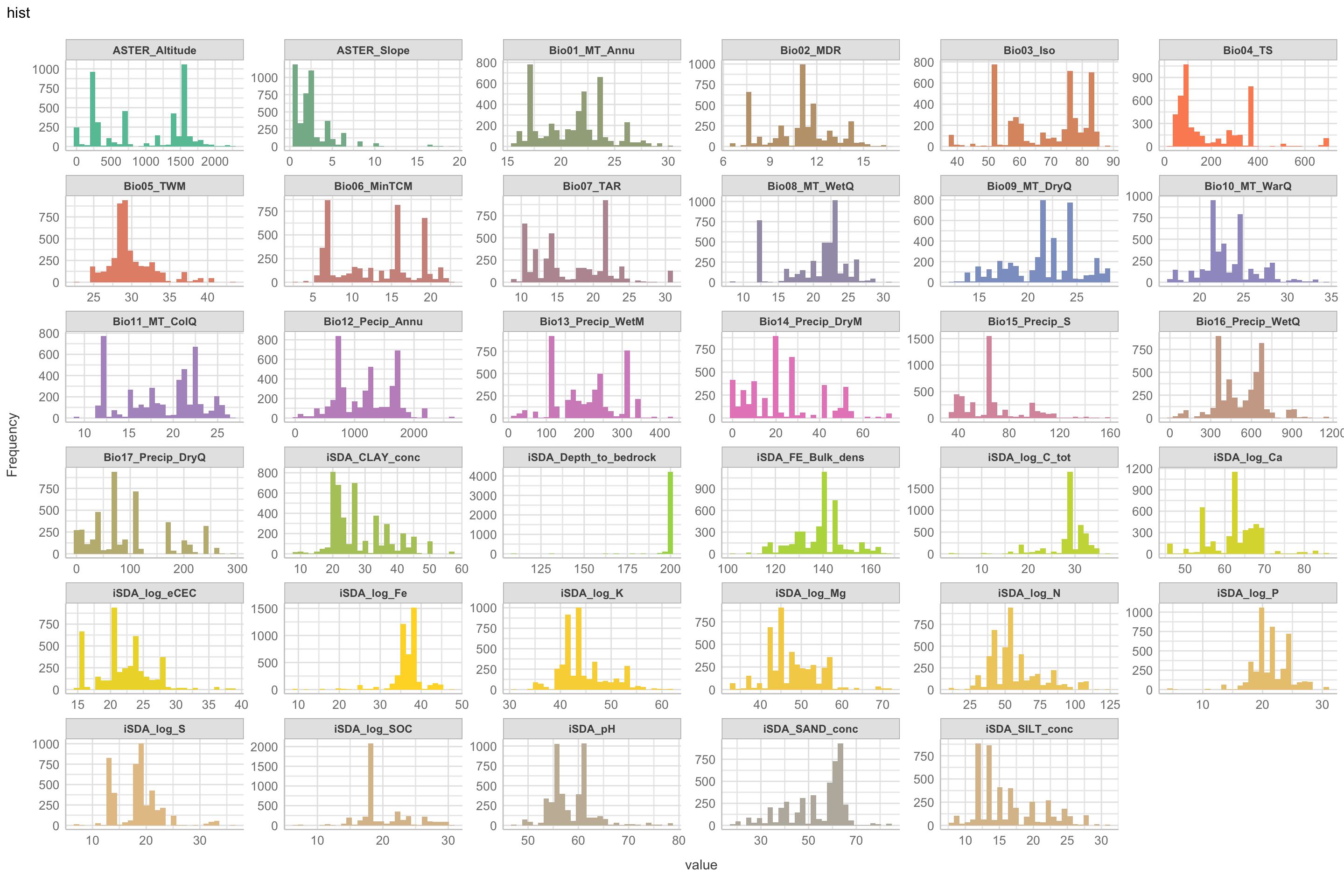
Figure 4: Histogram of biophysical predictors vs. logRR
Scatter plots i) of continuous predictors (all biophysical) i) of outcome (RR and logRR)
We use the plot_scatterplot() function from the DataExplorer package to generate a multiples of all the predictors with the response/outcome, logRR on the y-axis.
Show code
expl.agfor.scatter <- expl.agfor.data.no.na %>%
dplyr::select(-c("RR")) %>%
DataExplorer::plot_scatterplot(by = "logRR",
geom_point_args = list("col" = "#A2AC8A", "shape" = 10, "alpha" = 0.3,
"position" = "position_jitter"("width" = 0.1, "height" = 4.5), "size" = 0.3), # adding a jitter effect to avoid
ggtheme = theme_lucid(), # too much overlap of points
ncol = 6, nrow = 6,
title = "scatter")
# SAVING PLOT
saveRDS(expl.agfor.scatter, here::here("TidyMod_OUTPUT","expl.agfor.scatter.RDS"))
Show code
$page_1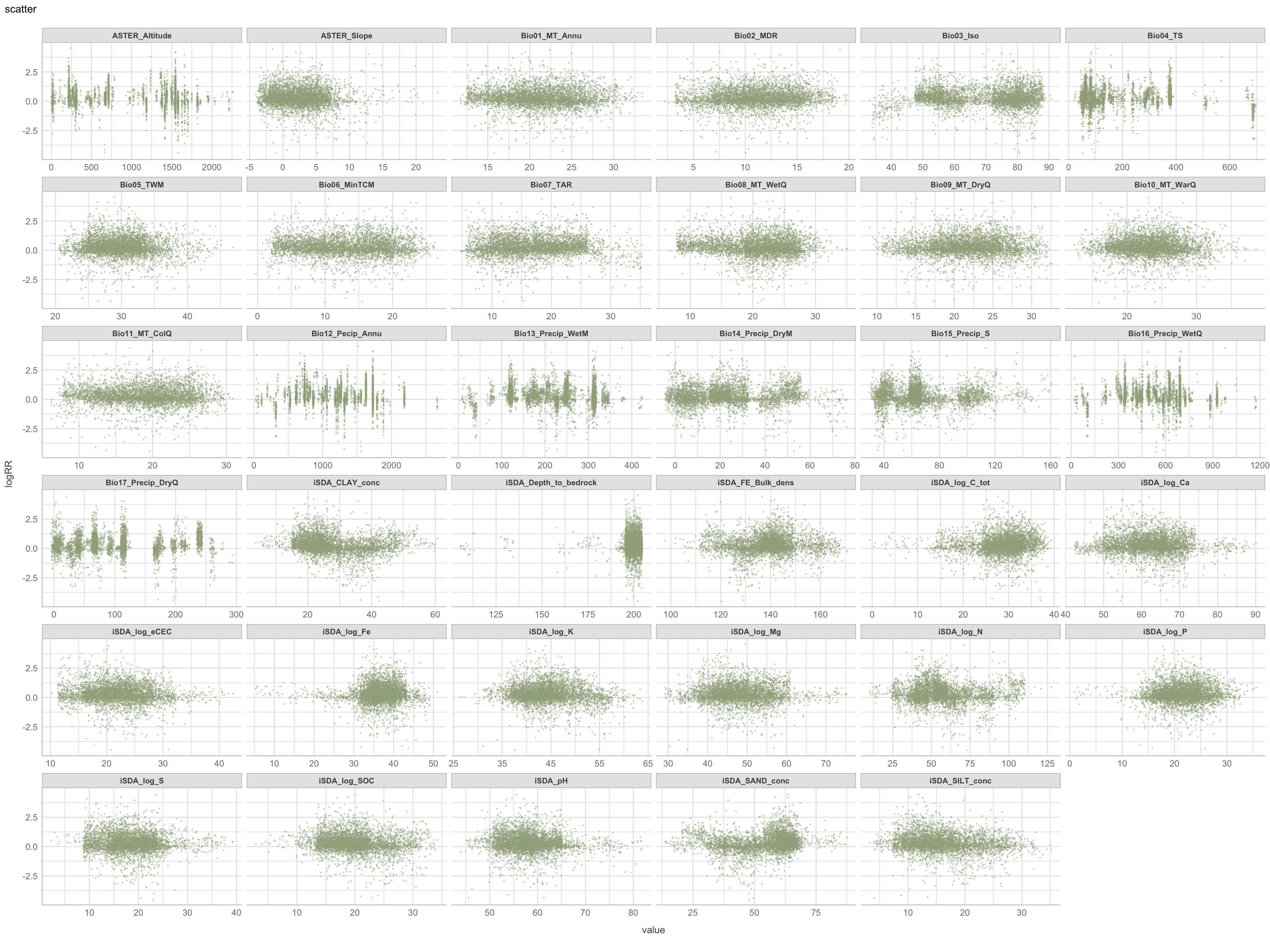
Figure 5: Scatter plot of biophysical predictors vs. logRR
Quantile-quantile plots i) of continuous predictors (all biophysical) i) of outcome (RR and logRR)
Quantile-quantile plots (QQ-plots) is a plot of the quantiles of one sample or distribution of the data against the quantiles of a second sample. QQ-plot makes it possible to compare the distribution of the data of a batch with the so-called normal or Gaussian distribution with the hypothesis that the data is distributed along the diagonal axis in the plot, through the 1st and 3rd quartiles (here shown in red).
expl.agfor.qqplot.pred <- expl.agfor.data.no.na %>%
dplyr::select(-c("RR", "logRR")) %>%
plot_qq(geom_qq_args = list("col" = "#A2AC8A", "shape" = 10, "alpha" = 0.3,
position = position_jitter(width = 0.1, height = 2), "size" = 0.3),
geom_qq_line_args = list("colour" = "#de2d26", "alpha" = 0.6, "size" = 0.4, "geom" = "path", "position" = "identity"),
ggtheme = theme_lucid(),
ncol = 6, nrow = 6,
title = "QQ plot")
# SAVING PLOT
saveRDS(expl.agfor.qqplot.pred, here::here("TidyMod_OUTPUT","expl.agfor.qqplot.pred.RDS"))
Show code
$page_1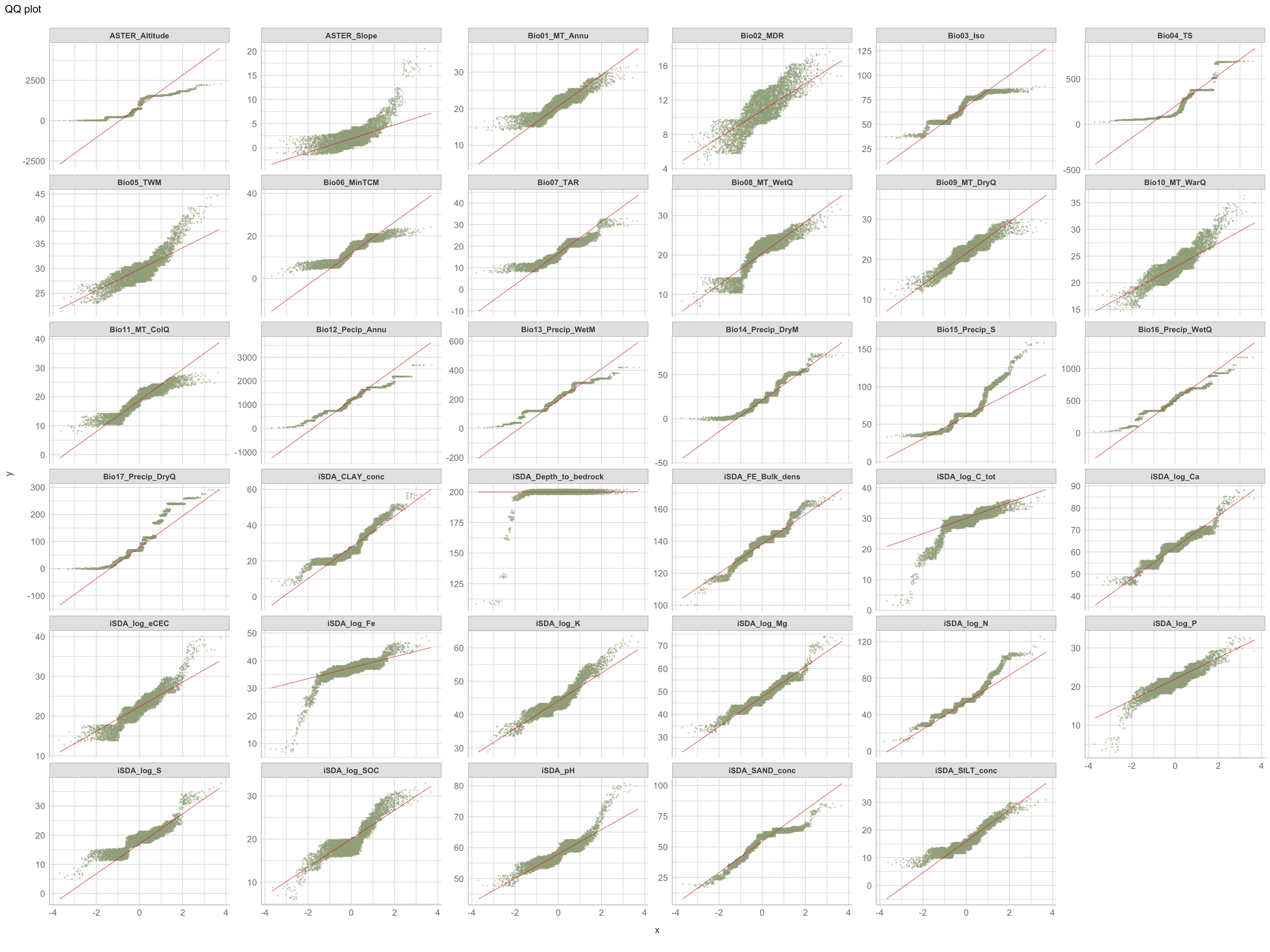
Figure 6: QQ plot of biophysical predictors
Again.. we clearly see that the predictors are not normally distributed. The QQ-plots can be interpreted based on whether there shape is of convex, concave, convex-concave, or concave-convex. A concave plot implies that the sample on the x-axis is more right-skewed, like the shape we see for iSDA Iron concentrations and iSDA total carbon. A convex plot implies that the sample on the x-axis is less right-skewed, or more left skewed, that is very clear what is the case for the slope feature. A convex-concave (concave-convex) plot implies that the data is heavy tailed on the x axis, e.g. iSDA soil organic carbon.
Lets also take a look at a QQ-plot for the outcome, logRR and RR.
expl.agfor.qqplot.logRR <- expl.agfor.data.no.na %>%
dplyr::select(c("RR", "logRR")) %>%
plot_qq(geom_qq_args = list("col" = "#FED82F", "shape" = 10, "alpha" = 0.3,
position = position_jitter(width = 0.1, height = 0.5), "size" = 0.5),
geom_qq_line_args = list("colour" = "#de2d26", "alpha" = 0.6, "size" = 0.6, "geom" = "path", "position" = "identity"),
ggtheme = theme_lucid(),
ncol = 2, nrow = 2,
title = "QQ plot")
# SAVING PLOT
saveRDS(expl.agfor.qqplot.logRR, here::here("TidyMod_OUTPUT","expl.agfor.qqplot.logRR.RDS"))
Show code
$page_1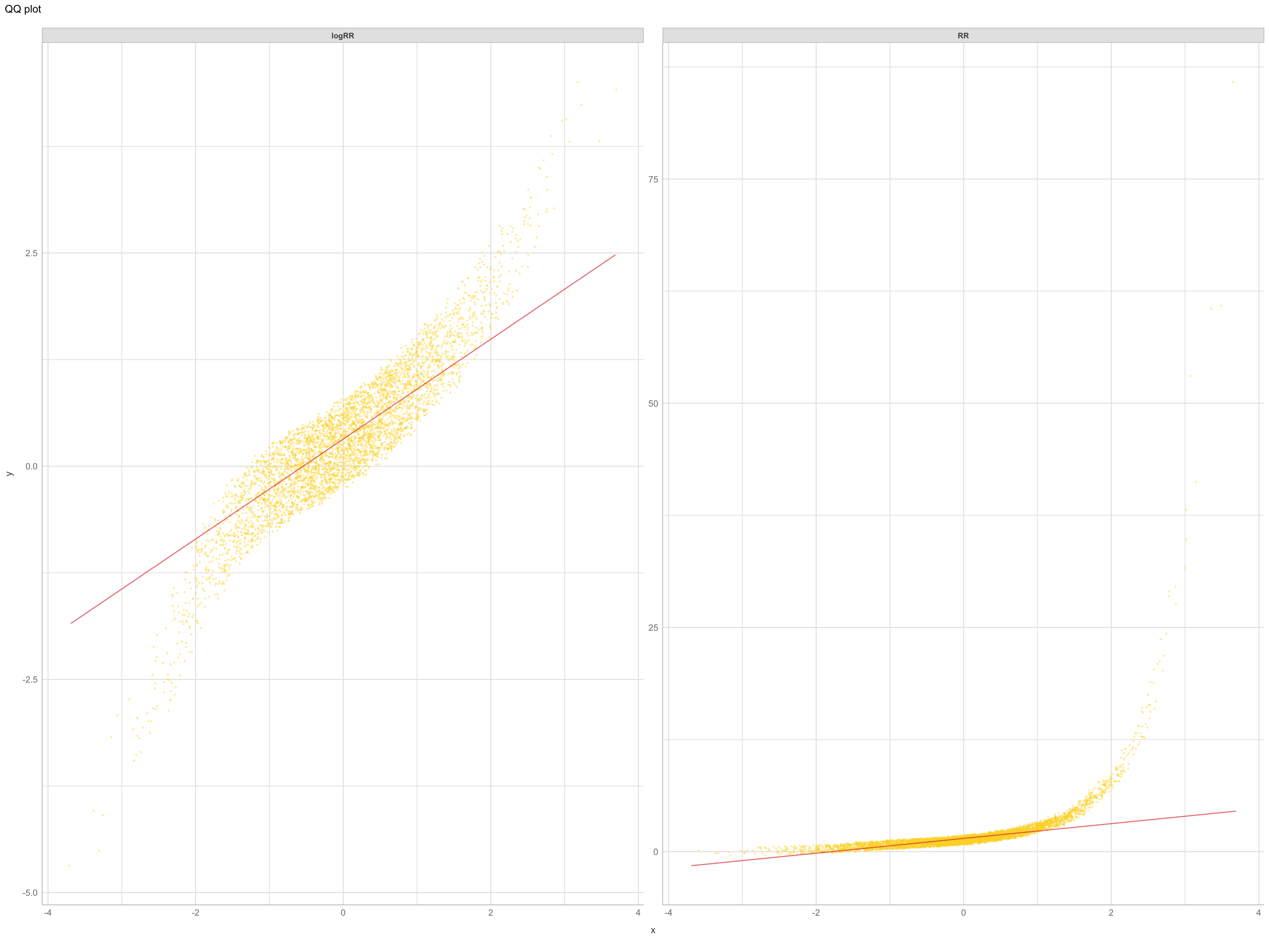
Figure 7: qq plot of outcomes RR and logRR
It is very evident again that the log-transformed RR has a better distribution, even though we can clearly see from the convex-concave patterns of logRR, that the data is heavy tailed on both ends. These “extreme” data points can perhabs be minimised with the removal of the extreme outliers, that we just discussed in previous section.
Discritization of target feature, logRR i) Boxplots of predictors vs. discritized logRR
We are now going to discretize our continues outcome feature, logRR into seven categorical/nominal groups. In statistics and machine learning, discretization refers to the process of converting or partitioning continuous features into discretized or nominal features with certain intervals. The goal of discretization is to reduce the number of values a continuous feature have by grouping it into a number of intervals or bins. This can be useful when one wish to perform EDA on a continues feature with no or very little linear (co)-relation to predictors. Hence, we can group the continuous outcome feature, logRR and look at discrete differences on the predictors for each group of logRR. Continuous features have a smaller chance of correlating with the target variable due to infinite degrees of freedom and may have a complex non-linear relationship. After discretizing logRR into groups it it easier to perform test on differences and for these results to be interpreted. The aim of performing the discretization of logRR in our case is to be able to make a pairwise t-test for the different groups of logRR. Thereby getting an understanding of whether there is significant differences between levels of logRR. Discretization, or binning/grouping of a continuous feature is mostly done in two ways, and we are going to evaluate the t-test outcome from both of these methods - because the binning technique is so different:
Equal-Width Discretization: Separating all possible values into ‘N’ number of bins, each having the same width. Formula for interval width: Width = (maximum value - minimum value) / N. Where N is the number of bins or intervals. This method doesn’t improve the value spread and it can handle outliers effectively.
Equal-Frequency Discretization: Separating all possible values into ‘N’ number of bins, each having the same amount of observations. These intervals are normally corresponding to ranges or quantile values. This method does improve the value spread and it can handle outliers effectively.
First, we are creating a two new feature columns in our agroforestry modelling data. We are using the functions cut_interval() and cut_number(), to perform the discrete levels of logRR based on the equal-frequency method and the equal-width method, respectfully. For each method seven groups are created. The groups range from 1, extremely low (low logRR values) to 7, extremely high (high logRR values).
# Pairwise comparison between PrName groups in the different biophysical co-variates.
#Do we find differences in logRR across ?
# Making new column in which we group the outcome variable logRR into binned categories
agrofor.biophys.modelling.data.discretized.logRR <- agrofor.biophys.modelling.data %>%
rationalize(logRR) %>%
drop_na(logRR) %>%
mutate(logRR_counts_cut_interval = cut_interval(logRR, n = 7)) %>%
mutate(logRR_EQR_group = case_when(
logRR_counts_cut_interval == "[-4.43,-3.16]" ~ "1.extremely_low",
logRR_counts_cut_interval == "(-3.16,-1.9]" ~ "2.very_low",
logRR_counts_cut_interval == "(-1.9,-0.627]" ~ "3.low",
logRR_counts_cut_interval == "(-0.627,0.642]" ~ "4.medium",
logRR_counts_cut_interval == "(0.642,1.91]" ~ "5.high",
logRR_counts_cut_interval == "(1.91,3.18]" ~ "6.very_high",
logRR_counts_cut_interval == "(3.18,4.45]" ~ "7.extremely_high",)) %>%
mutate(logRR_counts_cut_number = cut_number(logRR, n = 7)) %>%
mutate(logRR_EQNo_group = case_when(
logRR_counts_cut_number == "[-4.43,-0.31]" ~ "1.extremly_low",
logRR_counts_cut_number == "(-0.31,-0.0195]" ~ "2.very_low",
logRR_counts_cut_number == "(-0.0195,0.155]" ~ "3.low",
logRR_counts_cut_number == "(0.155,0.379]" ~ "4.medium",
logRR_counts_cut_number == "(0.379,0.643]" ~ "5.high",
logRR_counts_cut_number == "(0.643,1.1]" ~ "6.very_high",
logRR_counts_cut_number == "(1.1,4.45]" ~ "7.extremely_high",))
Lets compare the newly created factor levels. Are there differences in how logRR was grouped by the two methods..?
Show code
rmarkdown::paged_table(agrofor.biophys.modelling.data.discretized.logRR %>%
sample_n(25) %>% # randomly sampling a subset of 25 rows/observations
dplyr::relocate(logRR_EQNo_group, logRR_EQR_group, logRR, RR, ID))
Now we can prepare a parallel coordinate plot, that is an excellent way of visually assessing the differences in patterns for the discretized logRR groups for each of the biophysical predictors on the x-axis. A parallel coordinate plot allows to compare the feature of several individual observations (as a series) on a set of numeric variables (e.g. our biophysical predictors). We are going to make use of the ggparcoord() function from the GGally package to make this fancy multiples plot where all logRR groups are stacked on the y-axis.
Note: that we are making individual plots for each of the two discritization methods.
# Equal number data
par.coord.data.EQNo <-
agrofor.biophys.modelling.data.discretized.logRR %>%
dplyr::select(-c(ID, Out.SubInd, Product, MeanC, MeanT, AEZ16s, Latitude, Country, Longitude, Site.Type, Tree, SubPrName, RR,
logRR, logRR_EQR_group, PrName, PrName.Code, Out.SubInd.Code, logRR_counts_cut_interval, logRR_counts_cut_number)) %>%
mutate_if(is.character, as.factor) %>%
rationalize() %>%
drop_na() %>%
arrange(across(starts_with("logRR_EQNo_group")))
# Equal range data
par.coord.data.EQR <-
agrofor.biophys.modelling.data.discretized.logRR %>%
dplyr::select(-c(ID, Out.SubInd, Product, MeanC, MeanT, AEZ16s, Latitude, Country, Longitude, Site.Type, Tree, SubPrName, RR,
logRR, logRR_EQNo_group, PrName, PrName.Code, Out.SubInd.Code, logRR_counts_cut_interval, logRR_counts_cut_number)) %>%
mutate_if(is.character, as.factor) %>%
rationalize() %>%
drop_na() %>%
arrange(across(starts_with("logRR_EQR_group")))
# Facet label names
logRR_group.label.names <- c("1.extremely_low", "2.very_low", "3.low", "4.medium", "5.high", "6.very_high", "7.extremely_high")
names(logRR_group.label.names) <- c("1", "2", "3", "4", "5", "6", "7")
Defining a custom colours range for the parallel coordinate plots
Show code
# Defining a custom colours range
#library(RColorBrewer)
nb.cols.25 <- 25
era.af.colors.25 <- colorRampPalette(brewer.pal(8, "Set2"))(nb.cols.25)
Show code
par.coord.EQNo.plot <-
GGally::ggparcoord(par.coord.data.EQNo,
columns = 1:35,
#groupColumn = 36, # group by logRR_EQNo_group
scale = "center", # uniminmax to standardize vertical height, then center each variable at a value specified by the scaleSummary param
# order = "anyClass", # ordering by feature separation between any one class and the rest (as opposed to their overall variation between classes).
missing = "exclude",
showPoints = FALSE,
boxplot = FALSE,
#shadeBox = 35,
centerObsID = 1,
#title = "Discretized logRR values based on equal number vs. biophysical predictors",
alphaLines = 0.1,
splineFactor = TRUE, # making lines curvey
#shadeBox = NULL,
mapping = aes(color = as.factor(logRR_EQNo_group))) +
scale_color_manual("logRR_EQNo_group", labels = levels(par.coord.data.EQNo$logRR_EQNo_group), values = era.af.colors.25) +
# ggplot2::scale_color_manual(values = era.af.colors.25) + # assigning costom colour range
facet_grid(logRR_EQNo_group ~ . , labeller = labeller(logRR_EQNo_group = logRR_group.label.names)) +
coord_cartesian(ylim = c(- 0.8, 0.8)) +
theme_lucid() +
theme(plot.title = element_text(size = 20), legend.position = "none", #axis.text.x = element_text(angle = 60, hjust = 1)
axis.text.x = element_blank(),
strip.text.y = element_text(angle = 0),
plot.margin = margin(1, 0, 1, 0)) +
xlab("") +
ylab("")
Show code
# library(GGally)
par.coord.EQNo.plot.means <-
par.coord.data.EQNo %>%
dplyr::group_by(logRR_EQNo_group) %>%
dplyr::summarize_all(funs(mean)) %>%
ggparcoord(
columns=c(2:36),
# groupColumn = 1,
splineFactor = TRUE,
showPoints = TRUE,
#boxplot = TRUE,
#shadeBox = 4,
# scaleSummary = "mean",
scale = "center", # uniminmax to standardize vertical height, then center each variable at a value specified by the scaleSummary param
# order = "anyClass", # ordering by feature separation between any one class and the rest
missing = "exclude",
centerObsID = 1,
# title = "Discretized logRR values based on equal range vs. mean values of biophysical predictors",
alphaLines = 0.8,
mapping = aes(color = as.factor(logRR_EQNo_group), size = 3)) +
# mapping = ggplot2::aes(size = 3)) +
scale_color_manual("logRR_EQNo_group", labels = levels(par.coord.data.EQNo$logRR_EQNo_group), values = era.af.colors.25) +
# ggplot2::scale_color_manual(values = era.af.colors.25) + # assigning costom colour range
facet_grid(logRR_EQNo_group ~ . , labeller = labeller(logRR_EQNo_group = logRR_group.label.names)) +
coord_cartesian(ylim = c(- 2, 2)) +
theme_lucid() +
theme(plot.title = element_text(size = 20), axis.text.x = element_text(angle = 60, hjust = 1), legend.position = "none",
axis.title.x = element_blank(),
axis.title.y = element_blank(),
strip.text.y = element_text(angle = 0),
plot.margin = margin(0.5, 0, 0.5, 0))
#xlab("Mean values of biophysical predictors") +
#ylab("Uniminmax standardized logRR")
# Warnings to be ignored
# Warning: `funs()` was deprecated in dplyr 0.8.0.
# Please use a list of either functions or lambdas:
#
# # Simple named list:
# list(mean = mean, median = median)
#
# # Auto named with `tibble::lst()`:
# tibble::lst(mean, median)
#
# # Using lambdas
# list(~ mean(., trim = .2), ~ median(., na.rm = TRUE))
# This warning is displayed once every 8 hours.
# Call `lifecycle::last_warnings()` to see where this warning was generated.
Plotting the parallel coordinate plots of EQNo using the plot_grid() function from the cowplot package.
# Creating title
par.coord.EQNo.title <-
ggdraw() +
draw_label("Equal number discretized logRR vs biophysical predictors",
fontface = 'bold',
x = 0,
hjust = 0,
size = 20) +
theme(plot.margin = margin(5, 0, 0, 10))
# Using cowplot::plot_grid() to plot the two plots together and adding the title
par.coord.EQNo.combined <-
cowplot::plot_grid(
par.coord.EQNo.title,
NULL,
par.coord.EQNo.plot,
NULL,
par.coord.EQNo.plot.means,
#####
ncol = 1, nrow = 5,
align = "v",
axis = "l",
rel_widths = c(1),
rel_heights = c(0.4, 0.1, 4, 0.1, 4)) +
#perhaps reduce this for a bit more space
draw_label("Biophysical predictors", x = 0.63, y = 0, vjust = -0.9, angle = 0) +
draw_label("Uniminmax and centered standardized logRR", x = 0, y = 0.5, vjust = 1.5, angle = 90)
# SAVING PLOT
saveRDS(par.coord.EQNo.combined, here::here("TidyMod_OUTPUT","par.coord.EQNo.combined.RDS"))
Final parallel coordinate plot for the equal number discritized logRR
Show code
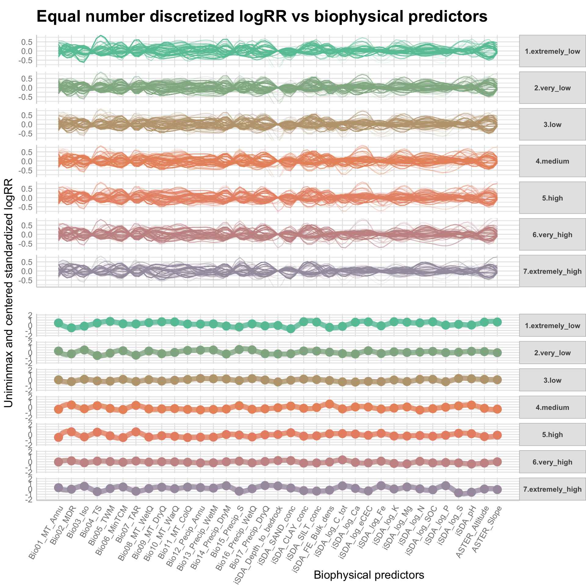
Figure 8: Parallel coordinate plots of discritized logRR against biophysical predictors, method: Equal number
We can use this parallel coordinate plot to get a better understanding of the non-linear relationship in our data. Initially, it does not seem like we have any noticeable differences in our predictors for the different factor levels of logRR. However, if we look carefully, some inconsistencies are present. For example, the predictor feature iSDA sand concentration seem to be more clear/precise for the higher values ou logRR and the influence of Bio16 precipitation of wettest quarter seems to diminish for the higher logRR factor groups. Reversely, we find that Bio03 isothermality is lower for the extremely low logRR group.
Let us now make a similar plot for the equal range method where logRR have been grouped based on their range.
Show code
par.coord.EQR.plot <-
ggparcoord(par.coord.data.EQR,
columns = 1:35,
#groupColumn = 36, # group by logRR_EQR_group
scale = "center", # uniminmax to standardize vertical height, then center each variable at a value specified by the scaleSummary param
# order = "anyClass", # ordering by feature separation between any one class and the rest (as opposed to their overall variation between classes).
missing = "exclude",
showPoints = FALSE,
boxplot = FALSE,
#shadeBox = 35,
centerObsID = 1,
#title = "Discretized logRR values based on equal number vs. biophysical predictors",
alphaLines = 0.1,
splineFactor = TRUE, # making lines curvey
#shadeBox = NULL,
mapping = aes(color = as.factor(logRR_EQR_group))) +
scale_color_manual("logRR_EQR_group", labels = levels(par.coord.data.EQR$logRR_EQR_group), values = era.af.colors.25) +
# ggplot2::scale_color_manual(values = era.af.colors.25) + # assigning costom colour range
facet_grid(logRR_EQR_group ~ . , labeller = labeller(logRR_EQR_group = logRR_group.label.names)) +
coord_cartesian(ylim = c(- 0.8, 0.8)) +
theme_lucid() +
theme(plot.title = element_text(size = 20), legend.position = "none", #axis.text.x = element_text(angle = 60, hjust = 1)
axis.text.x = element_blank(),
strip.text.y = element_text(angle = 0),
plot.margin = margin(1, 0, 1, 0)) +
xlab("") +
ylab("")
Plotting the parallel coordinate plots of EQR using the plot_grid() function from the cowplot package.
Show code
par.coord.EQR.plot.means <-
par.coord.data.EQR %>%
dplyr::group_by(logRR_EQR_group) %>%
dplyr::summarize_all(funs(mean)) %>%
ggparcoord(
columns=c(2:36),
# groupColumn = 1,
splineFactor = TRUE,
showPoints = TRUE,
#boxplot = TRUE,
#shadeBox = 4,
# scaleSummary = "mean",
scale = "center", # uniminmax to standardize vertical height, then center each variable at a value specified by the scaleSummary param
# order = "anyClass", # ordering by feature separation between any one class and the rest
missing = "exclude",
centerObsID = 1,
# title = "Discretized logRR values based on equal range vs. mean values of biophysical predictors",
alphaLines = 0.8,
mapping = aes(color = as.factor(logRR_EQR_group), size = 3)) +
# mapping = ggplot2::aes(size = 3)) +
scale_color_manual("logRR_EQR_group", labels = levels(par.coord.data.EQR$logRR_EQR_group), values = era.af.colors.25) +
# ggplot2::scale_color_manual(values = era.af.colors.25) + # assigning costom colour range
facet_grid(logRR_EQR_group ~ . , labeller = labeller(logRR_EQR_group = logRR_group.label.names)) +
coord_cartesian(ylim = c(- 2, 2)) +
theme_lucid() +
theme(plot.title = element_text(size = 20), axis.text.x = element_text(angle = 60, hjust = 1), legend.position = "none",
axis.title.x = element_blank(),
axis.title.y = element_blank(),
strip.text.y = element_text(angle = 0),
plot.margin = margin(0.5, 0, 0.5, 0))
#xlab("Mean values of biophysical predictors") +
#ylab("Uniminmax standardized logRR")
Cowplot of EQR
# Creating title
par.coord.EQR.title <-
ggdraw() +
draw_label("Equal range discretized logRR vs biophysical predictors",
fontface = 'bold',
x = 0,
hjust = 0,
size = 20) +
theme(plot.margin = margin(5, 0, 0, 10))
# Using cowplot::plot_grid() to plot the two plots together and adding the title
par.coord.EQR.combined <-
cowplot::plot_grid(
par.coord.EQR.title,
NULL,
par.coord.EQR.plot,
NULL,
par.coord.EQR.plot.means,
#####
ncol = 1, nrow = 5,
align = "v",
axis = "l",
rel_widths = c(1),
rel_heights = c(0.4, 0.1, 4, 0.1, 4)) +
#perhaps reduce this for a bit more space
draw_label("Biophysical predictors", x = 0.63, y = 0, vjust = -0.9, angle = 0) +
draw_label("Uniminmax and centered standardized logRR", x = 0, y = 0.5, vjust = 1.5, angle = 90)
# SAVING PLOT
saveRDS(par.coord.EQR.combined, here::here("TidyMod_OUTPUT","par.coord.EQR.combined.RDS"))
Final parallel coordinate plot for the equal range discritized logRR
Show code
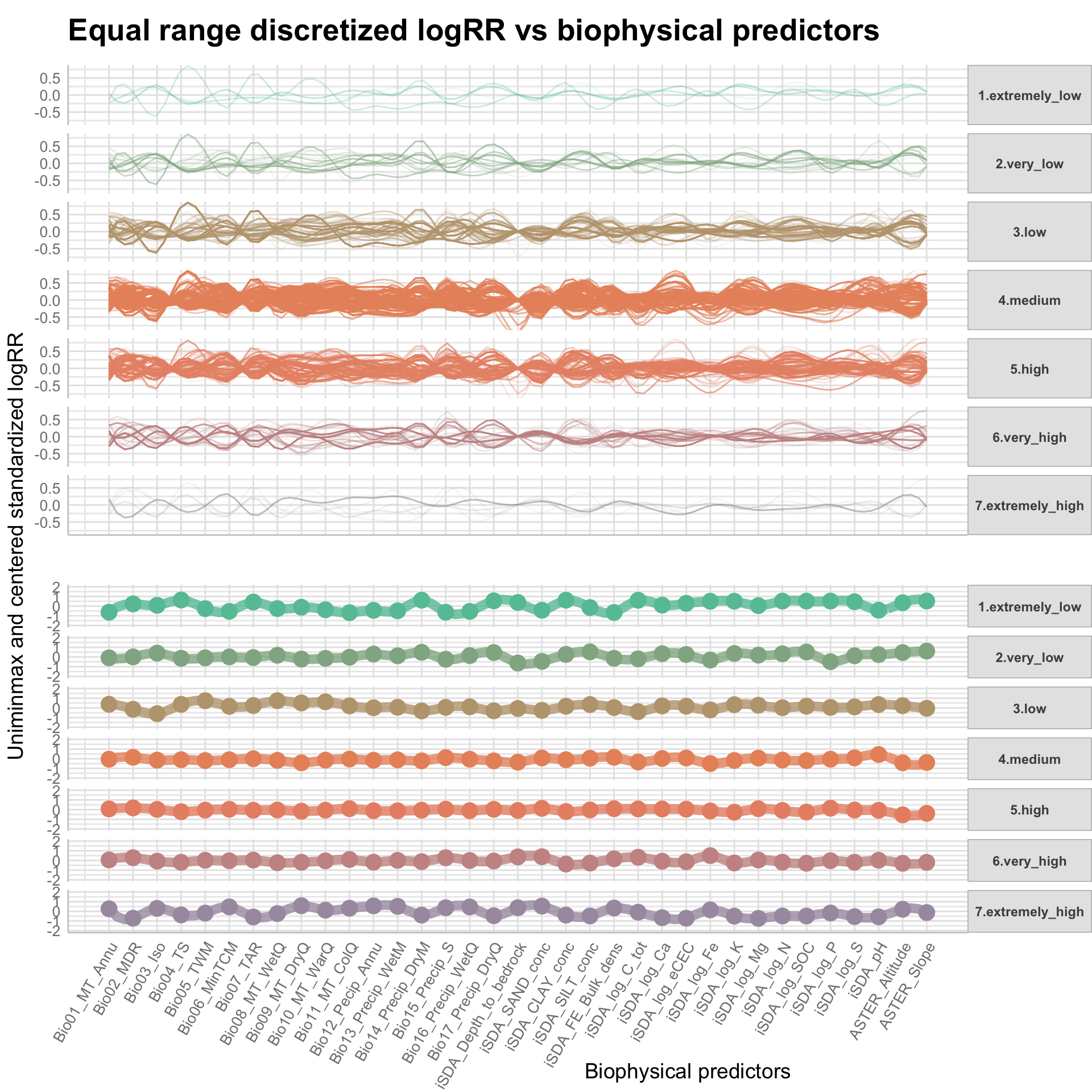
Figure 9: Parallel coordinate plots of discritized logRR against biophysical predictors, method: Equal range
With the equal range method we have the downside that we have fewer observation in the extreme low and extreme high regions. This might create some bias when interpreting the plots. The interesting aspect of these plots is that we do see differences among and between the discretized logRR values for the different biophysical variables, suggesting that logRR is associated with (the combination of) biophysical co-variables.
Boxplots of predictors vs. discritized logRR
We will use the plot_boxplot() function from the DataExplorer package to create a multiples plot of boxplots for each continuous feature based on the outcome, logRR feature. Boxplots are powerful EDA visuals as they are very intuitivly showing where the most of the data is (inside of the box), and whether variables have \(many\) outliers or not. Boxplots are also useful for a quick comparison of data distributions across groups, samples or categories, because they visualize center, spread and range of every group. Thus, similarly to the correlation analysis we did above, boxplots also help to develop hypotheses.
Generating custom colour object with 180 colours
Show code
# 180 levels of 35 colours
explor.cols.group.35_180 <- c("#66C2A5", "#66C2A5", "#66C2A5", "#66C2A5", "#66C2A5",
"#84B797", "#84B797", "#84B797", "#84B797", "#84B797",
"#A2AC8A", "#A2AC8A", "#A2AC8A", "#A2AC8A", "#A2AC8A",
"#C0A27C", "#C0A27C", "#C0A27C", "#C0A27C", "#C0A27C",
"#DE976F", "#DE976F", "#DE976F", "#DE976F", "#DE976F",
"#FC8D62", "#FC8D62", "#FC8D62", "#FC8D62", "#FC8D62",
"#E59077", "#E59077", "#E59077", "#E59077", "#E59077",
"#CF948C", "#CF948C", "#CF948C", "#CF948C", "#CF948C",
"#B998A1", "#B998A1", "#B998A1", "#B998A1", "#B998A1",
"#A39CB5", "#A39CB5", "#A39CB5", "#A39CB5", "#A39CB5",
"#8DA0CB", "#8DA0CB", "#8DA0CB", "#8DA0CB", "#8DA0CB",
"#9F9BC9", "#9F9BC9", "#9F9BC9", "#9F9BC9", "#9F9BC9",
"#B197C7", "#B197C7", "#B197C7", "#B197C7", "#B197C7",
"#C392C6", "#C392C6", "#C392C6", "#C392C6", "#C392C6",
"#D48EC4", "#D48EC4", "#D48EC4", "#D48EC4", "#D48EC4",
"#E78AC3", "#E78AC3", "#E78AC3", "#E78AC3", "#E78AC3",
"#DA99AC", "#DA99AC", "#DA99AC", "#DA99AC", "#DA99AC",
"#CDA996", "#CDA996", "#CDA996", "#CDA996", "#CDA996",
"#C0B880", "#C0B880", "#C0B880", "#C0B880", "#C0B880",
"#B3C86A", "#B3C86A", "#B3C86A", "#B3C86A", "#B3C86A",
"#A6D854", "#A6D854", "#A6D854", "#A6D854", "#A6D854",
"#B7D84C", "#B7D84C", "#B7D84C", "#B7D84C", "#B7D84C",
"#C9D845", "#C9D845", "#C9D845", "#C9D845", "#C9D845",
"#DBD83D", "#DBD83D", "#DBD83D", "#DBD83D", "#DBD83D",
"#EDD836", "#EDD836", "#EDD836", "#EDD836", "#EDD836",
"#FED82F", "#FED82F", "#FED82F", "#FED82F", "#FED82F",
"#F9D443", "#F9D443", "#F9D443", "#F9D443", "#F9D443",
"#F4D057", "#F4D057", "#F4D057", "#F4D057", "#F4D057",
"#EFCC6B", "#EFCC6B", "#EFCC6B", "#EFCC6B", "#EFCC6B",
"#EAC87F", "#EAC87F", "#EAC87F", "#EAC87F", "#EAC87F",
"#E5C494", "#E5C494", "#E5C494", "#E5C494", "#E5C494",
"#DBC09A", "#DBC09A", "#DBC09A", "#DBC09A", "#DBC09A",
"#C7B9A6", "#C7B9A6", "#C7B9A6", "#C7B9A6", "#C7B9A6",
"#BCB6AC", "#BCB6AC", "#BCB6AC", "#BCB6AC", "#BCB6AC",
"#DBC09A", "#DBC09A", "#DBC09A", "#DBC09A", "#DBC09A"
)
expl.agfor.boxplot.pred <- expl.agfor.data.no.na %>%
dplyr::select(-c("RR")) %>%
plot_boxplot(by = "logRR",
geom_boxplot_args = list("outlier.color" = "#636363", "outlier.shape" = 1, "outlier.size" = 0.4, "alpha" = 0.6,
"fill" = (explor.cols.group.35_180)),
ggtheme = theme_lucid(), ncol = 6, nrow = 6,
title = "Boxplots of predictors vs. discritized logRR")
# SAVING PLOT
saveRDS(expl.agfor.boxplot.pred, here::here("TidyMod_OUTPUT","expl.agfor.boxplot.pred.RDS"))
Show code
$page_1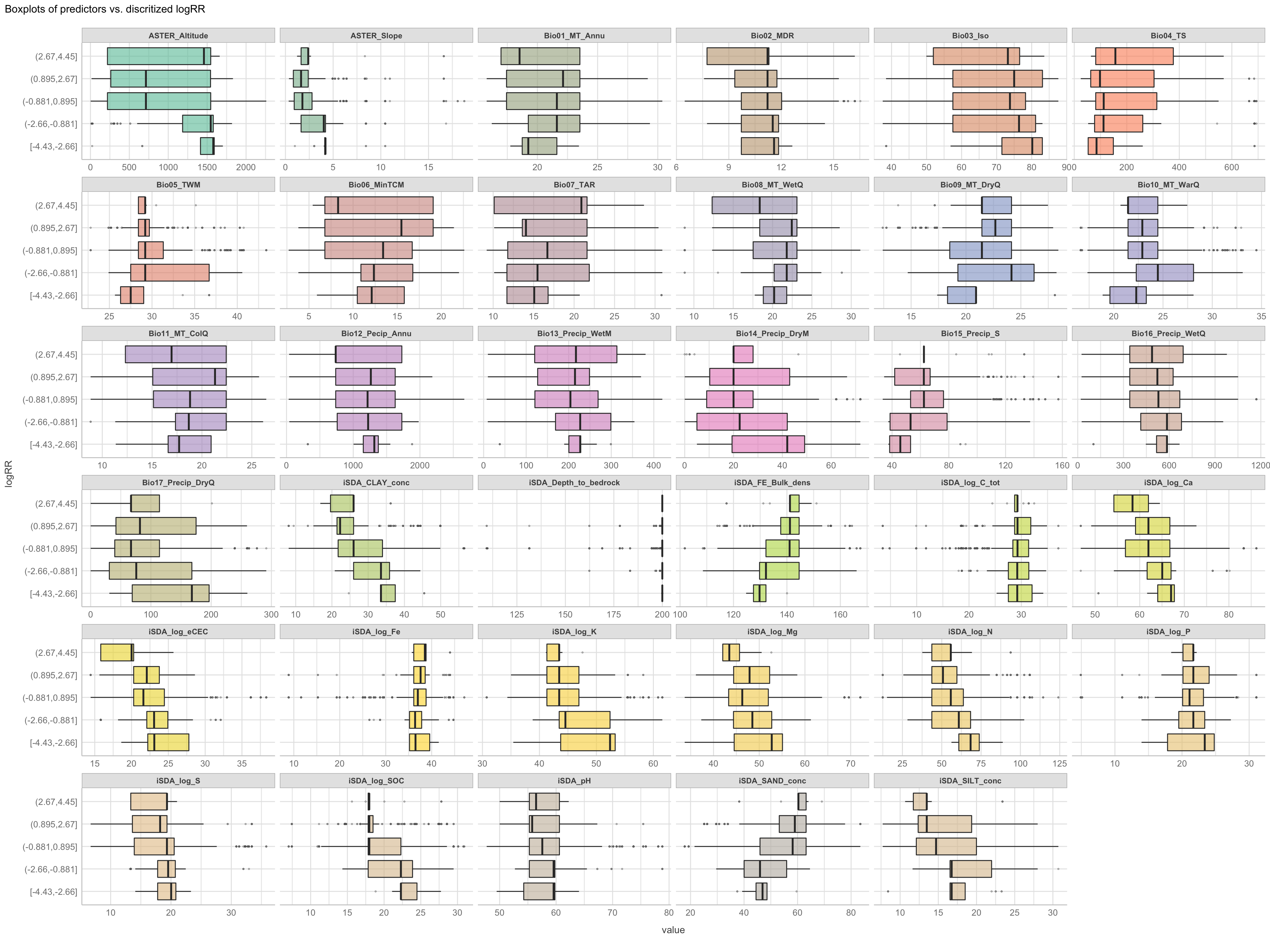
Figure 10: Boxplots of predictors and discretized logRR
The multiples plot above is showing each of the biophysical predictorsin separate plots as we have seen before. The novelty and slightly unusual aspects of the plot above, is that we have depicted our continuous outcome variable, logRR in a discretized manner on the y axis and shown the range of the respected biophysical predictor on the x-axis. The groupings, also called bins, of logRR for each of the biophysical predictors shows some promising trends: That we do see differences in thhe predictors for different levels of our discretized logRR outcome. This is good news as these differences in the data can be used by our machine learning models. In addition, we also see that we have a large amount of outliers (Note: 1.5 * IQR), especially in the central/median groups.
Multiple pairwise t-test using discritized logRR values
Using equal range discritized logRR groups we can test for significant difference between the groups of logRR values. This is interesting because we can use it to quickly estimate whether logRR values are in fact statistically significantly different from each other. If not it might be very difficult to distingush them and the influence our biophysical predictors might have/have not on the logRR.
We know a standard paired t-test, that is used to check the difference between a group of two members (only between two groups). The multiple t-test can be used to performs many t-tests simultaneously, with each test comparing two groups of data. This is practical as we in our case are mostly interested in a EDA of how individual “artificially” discritized groups of our outcome feature, logRR is different from other groups. The multiple pairwise t-test is performed in following steps:
Creating a long format of the agroforestry data where logRR have been discritized (either equal range or equal number method)
Selecting the
Transforming data into long format
# Transform the data into long format
# Put all variables in the same column except `logRR_EQR_group`, the grouping variable
####################################################################################################################
# Discretized with equal number
agrofor.biophys.modelling.data.long.EQNo <-
agrofor.biophys.modelling.data.discretized.logRR %>%
dplyr::select(Bio01_MT_Annu:logRR_EQNo_group) %>%
rationalize() %>%
drop_na() %>%
dplyr::select(-(c("RR", "logRR", "logRR_counts_cut_interval", "logRR_EQR_group" , "logRR_counts_cut_number"))) %>%
mutate_if(is.character, as.factor) %>%
pivot_longer(-logRR_EQNo_group, names_to = "variables", values_to = "value")
####################################################################################################################
# Discretized with equal range
agrofor.biophys.modelling.data.long.EQR <-
agrofor.biophys.modelling.data.discretized.logRR %>%
dplyr::select(Bio01_MT_Annu:logRR_EQR_group) %>%
rationalize() %>%
drop_na() %>%
dplyr::select(-(c("RR", "logRR", "logRR_counts_cut_interval"))) %>%
mutate_if(is.character, as.factor) %>%
pivot_longer(-logRR_EQR_group, names_to = "variables", values_to = "value")
dim(agrofor.biophys.modelling.data.long.EQR)
# [1] 156135 3
dim(agrofor.biophys.modelling.data.long.EQNo)
# [1] 156135 3
Creating summerised statistics
####################################################################################################################
# Summary statistics -- Equal number
agrofor.biophys.modelling.data.long.EQNo.stats <-
agrofor.biophys.modelling.data.long.EQNo %>%
group_by(variables, logRR_EQNo_group) %>%
summarise(
n = n(),
mean = mean(value),
sd = sd(value)
) %>%
ungroup()
####################################################################################################################
# Summary statistics -- Equal range
agrofor.biophys.modelling.data.long.EQR.stats <-
agrofor.biophys.modelling.data.long.EQR %>%
group_by(variables, logRR_EQR_group) %>%
summarise(
n = n(),
mean = mean(value),
sd = sd(value)
) %>%
ungroup()
# `summarise()` has grouped output by 'variables'. You can override using the `.groups` argument.
# `summarise()` has grouped output by 'variables'. You can override using the `.groups` argument.
# SAVING LONG DATA
saveRDS(agrofor.biophys.modelling.data.long.EQNo.stats, here::here("TidyMod_OUTPUT", "agrofor.biophys.modelling.data.long.EQNo.stats.RDS"))
saveRDS(agrofor.biophys.modelling.data.long.EQR.stats, here::here("TidyMod_OUTPUT", "agrofor.biophys.modelling.data.long.EQR.stats.RDS"))
Show code
agrofor.biophys.modelling.data.long.EQNo.stats <- readRDS( here::here("TidyMod_OUTPUT","agrofor.biophys.modelling.data.long.EQNo.stats.RDS"))
rmarkdown::paged_table(agrofor.biophys.modelling.data.long.EQNo.stats %>% sample_n(25))
Show code
agrofor.biophys.modelling.data.long.EQR.stats <- readRDS( here::here("TidyMod_OUTPUT","agrofor.biophys.modelling.data.long.EQR.stats.RDS"))
rmarkdown::paged_table(agrofor.biophys.modelling.data.long.EQR.stats %>% sample_n(25))
This long data format is full of potential because we can use it to group our rows/observations based on the discretized logRR factor levels - and this will conglomerate the variables–value combinations. Thereby allowing for a pairwise t-test between the logRR factor levels for each of the different biophysical predictor features. We can use this to for example ask the question: Is there (significant) differences between the logRR factor levels when it comes to precipitation (BIO13, BIO14, BIO15, BIO16, BIO17, BIO18 and BIO19). If there is differences it can indicate that precipitation or any given predictor can be used to predict logRR values. Note that caution has to be made when interpretation the discritized logRR factor levels because any continuous features have a smaller chance of correlating with the target variable due to the concept of infinite degrees of freedom thus the categorical continuous version of logRR may have a complex non-linear relationship and conclusions from the discretized logRR cannot be directly transferred to the continuous logRR.
Ultimately we are interested in predicting logRR in a continuous version, hence we want to approach the machine learning as a regression problem. Yet, we could also use a classification approach on discretized logRR levels. When we discretize an outcome feature that we want to predict, we are fitting it to bins hence reducing the impact of small fluctuation in the data, considered as noise. This noise is reduced through discretization. Another advantage of discretizing the outcome feature, logRR would be that often, it is easier to understand continuous data (such as logRR) when its divided and stored into meaningful categories or groups. For example, we could divide out predicted logRR values into the following groups: High logRR (large benefit of agroforestry - compared to control practice), medium logRR (intermediate/no benefit of agroforestry - compared to control practice) and low logRR (negative impacts of agroforestry - compared to control practice).
That was a little side note. Let us now run the multiple pairwise t-test analysis for the different logRR factor levels in which we compare the differences in the biophysical predictors across the seven groups of logRR. We are using the rstatix package functions t_test()
Multiple pairwise t-test using discritized logRR values i) of continuous predictors (all biophysical)
Group the data by variables and compare logRR groups with t-tests add significance levels
# Group the data by variables and compare logRR groups with t-tests add significance levels
####################################################################################################################
# With equal number discritization
agrofor.biophys.modelling.data.long.stat.ttest.EQNo <- agrofor.biophys.modelling.data.long.EQNo %>%
group_by(variables) %>%
rstatix::t_test(value ~ logRR_EQNo_group, p.adjust.method = "BH") # adjusting p-values based on the Benjamini-Hochberg method
# Remove unnecessary columns, arranging the columns neatly and display the outputs
agrofor.biophys.modelling.data.long.stat.ttest.EQNo.results <- agrofor.biophys.modelling.data.long.stat.ttest.EQNo %>%
select(-.y., -statistic, -df) %>%
relocate(variables, group1, group2, p, p.adj.signif) %>%
dplyr::arrange(desc(-p))
####################################################################################################################
# With equal range discritization
agrofor.biophys.modelling.data.long.stat.ttest.EQR <- agrofor.biophys.modelling.data.long.EQR %>%
group_by(variables) %>%
rstatix::t_test(value ~ logRR_EQR_group, p.adjust.method = "BH") # adjusting p-values based on the Benjamini-Hochberg method
# Remove unnecessary columns, arranging the columns neatly and display the outputs
agrofor.biophys.modelling.data.long.stat.ttest.EQR.results <- agrofor.biophys.modelling.data.long.stat.ttest.EQR %>%
select(-.y., -statistic, -df) %>%
relocate(variables, group1, group2, p, p.adj.signif) %>%
dplyr::arrange(desc(-p))
# SAVING LONG DATA
saveRDS(agrofor.biophys.modelling.data.long.stat.ttest.EQNo.results, here::here("TidyMod_OUTPUT", "agrofor.biophys.modelling.data.long.stat.ttest.EQNo.results.RDS"))
saveRDS(agrofor.biophys.modelling.data.long.stat.ttest.EQR.results, here::here("TidyMod_OUTPUT", "agrofor.biophys.modelling.data.long.stat.ttest.EQR.results.RDS"))
Lets look at the (significant) differences between our discretized logRR groups for the equal number method
Show code
agrofor.biophys.modelling.data.long.stat.ttest.EQNo.results <- readRDS( here::here("TidyMod_OUTPUT","agrofor.biophys.modelling.data.long.stat.ttest.EQNo.results.RDS"))
rmarkdown::paged_table(agrofor.biophys.modelling.data.long.stat.ttest.EQNo.results)
..and now for the equal range method
Show code
agrofor.biophys.modelling.data.long.stat.ttest.EQR.results <- readRDS( here::here("TidyMod_OUTPUT","agrofor.biophys.modelling.data.long.stat.ttest.EQR.results.RDS"))
rmarkdown::paged_table(agrofor.biophys.modelling.data.long.stat.ttest.EQR.results)
We find that there is significant differences between discretized logRR groups, this is the case for both methods of equal and equal number.
Before we visualise these trends we are first going to generating the mean values of all biophysical variables that we can add to the boxplot as a vertical reference bar. Open the code by pressing “Show code” to see how thiswas done.
Show code
####################################################################################################################
# Mean values for each biophysical variable -- With equal number discritization
agfor.biophys.mean.EQNo <- agrofor.biophys.modelling.data.long.EQNo.stats %>%
group_by(variables) %>%
dplyr::summarise(mean) %>%
pivot_wider(names_from = variables, values_from = mean, values_fn = mean) %>%
pivot_longer(cols = everything(), names_to = "variables", values_to = "mean.values")
####################################################################################################################
# Mean values for each biophysical variable -- With equal range discritization
agfor.biophys.mean.EQR <- agrofor.biophys.modelling.data.long.EQR.stats %>%
group_by(variables) %>%
dplyr::summarise(mean) %>%
pivot_wider(names_from = variables, values_from = mean, values_fn = mean) %>%
pivot_longer(cols = everything(), names_to = "variables", values_to = "mean.values")
#`summarise()` has grouped output by 'variables'. You can override using the `.groups` argument.
# `summarise()` has grouped output by 'variables'. You can override using the `.groups` argument.
Let us define the mean values to be depicted in the boxplot be merging with the datasets.
####################################################################################################################
# Horizontal line based on mean values for each biophysical variable -- With equal number discritization
agrofor.biophys.long.EQNo.hline <- merge(agrofor.biophys.modelling.data.long.EQNo,
agfor.biophys.mean.EQNo,
by.x = "variables", by.y = "variables")
####################################################################################################################
# Horizontal line based on mean values for each biophysical variable -- With equal range discritization
agrofor.biophys.long.EQR.hline <- merge(agrofor.biophys.modelling.data.long.EQR,
agfor.biophys.mean.EQR,
by.x = "variables", by.y = "variables")
Defining a custom colours range for the boxplots
Show code
# Colour range with 35 levels
nb.cols.35 <- 35
era.af.colors.35 <- colorRampPalette(brewer.pal(8, "Set2"))(nb.cols.35)
Create multi-panel Boxplots with t-test p-values for the EQNo
# Create multi-panel Boxplots with t-test p-values
logRR.EQNo.group.comparisons <- list(c("1.extremely_low", "2.very_low"),
c("2.very_low", "3.low"),
c("3.low", "4.medium"),
c("4.medium", "5.high"),
c("5.high", "6.very_high"),
c("6.very_high", "7.extremely_high"),
c("7.extremely_high", "1.extremely_low"))
ttest.pair.plot.discretized.logRR.biophy.pred.EQNo <- ggpubr::ggboxplot(agrofor.biophys.long.EQNo.hline,
"logRR_EQNo_group", "value",
color = "variables", palette = era.af.colors.35, add = "jitter", add.params = list(size = 0.2, jitter = 0.3),
title = "Differences in discretized logRR values based on equal number, for each biophysical predictor",
bxp.errorbar = TRUE, bxp.errorbar.width = 0.5, outlier.shape = 10) +
facet_wrap(variables ~ ., scales = "free_y") +
theme_lucid() +
theme(plot.title = element_text(size = 20), axis.text.x = element_text(angle = 60, hjust = 1), legend.position = "none") +
xlab("Biophysical co-variates/predictors") +
ylab("logRR") +
font("title", size = 20, color = "black") +
geom_hline(aes(yintercept = mean.values), linetype = 2) +
scale_y_continuous(expand = expansion(mult = c(0, 0.2))) +
stat_compare_means(comparisons = logRR.EQNo.group.comparisons,
mapping = aes(label = sprintf("p = %1.1f", as.numeric(..p.format..))), color = "black", size = 2.5) +
stat_compare_means(label = "p.signif", method = "t.test", ref.group = ".all.", label.y = 10)
# stat_compare_means(method = "anova", label.y = - 5, mapping = aes(label = sprintf("p = %1.1f", as.numeric(..p.format..))), size = 2.0) +
# Using `as.character()` on a quosure is deprecated as of rlang 0.3.0.
# Please use `as_label()` or `as_name()` instead.
# This warning is displayed once per session.
# SAVING PLOT
saveRDS(ttest.pair.plot.discretized.logRR.biophy.pred.EQNo, here::here("TidyMod_OUTPUT", "ttest.pair.plot.discretized.logRR.biophy.pred.EQNo.RDS"))
Create multi-panel Boxplots with t-test p-values for the EQR
# Create multi-panel Boxplots with t-test p-values
logRR.EQR.group.comparisons <- list(c("1.extremely_low", "2.very_low"),
c("2.very_low", "3.low"),
c("3.low", "4.medium"),
c("4.medium", "5.high"),
c("5.high", "6.very_high"),
c("6.very_high", "7.extremely_high"),
c("7.extremely_high", "1.extremely_low"))
ttest.pair.plot.discretized.logRR.biophy.pred.EQR <- ggpubr::ggboxplot(agrofor.biophys.long.EQR.hline,
"logRR_EQR_group", "value",
color = "variables", palette = era.af.colors.35, add = "jitter", add.params = list(size = 0.2, jitter = 0.3),
title = "Differences in discretized logRR values based on equal range, for each biophysical predictor",
bxp.errorbar = TRUE, bxp.errorbar.width = 0.5, outlier.shape = 10) +
facet_wrap(variables ~ ., scales = "free_y") +
theme_lucid() +
theme(plot.title = element_text(size = 20), axis.text.x = element_text(angle = 60, hjust = 1), legend.position = "none") +
xlab("Biophysical co-variates/predictors") +
ylab("logRR") +
font("title", size = 20, color = "black") +
geom_hline(aes(yintercept = mean.values), linetype = 2) +
scale_y_continuous(expand = expansion(mult = c(0, 0.2))) +
stat_compare_means(comparisons = logRR.EQR.group.comparisons,
mapping = aes(label = sprintf("p = %1.1f", as.numeric(..p.format..))), color = "black", angle = -90, size = 2.5) +
stat_compare_means(label = "p.signif", method = "t.test", ref.group = ".all.", label.y = 10)
# stat_compare_means(method = "anova", label.y = - 5, mapping = aes(label = sprintf("p = %1.1f", as.numeric(..p.format..))), size = 2.0) +
# Using `as.character()` on a quosure is deprecated as of rlang 0.3.0.
# Please use `as_label()` or `as_name()` instead.
# This warning is displayed once per session.
# SAVING PLOT
saveRDS(ttest.pair.plot.discretized.logRR.biophy.pred.EQR, here::here("TidyMod_OUTPUT", "ttest.pair.plot.discretized.logRR.biophy.pred.EQR.RDS"))
Boxplot of equal range discretized logRR vs. biophysical predictors
Show code
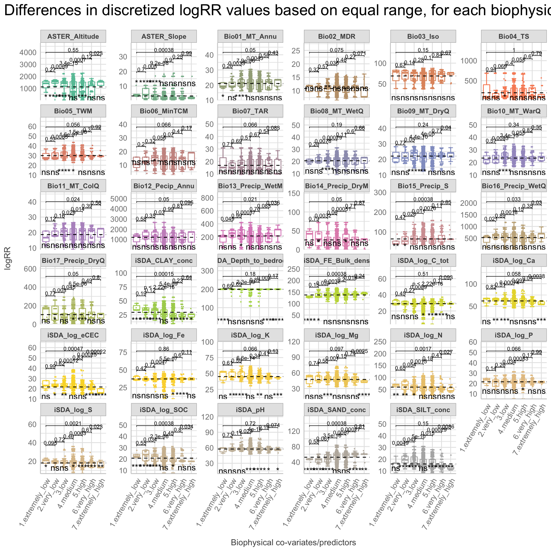
Figure 11: Boxplot of equal range discretized logRR vs. biophysical predictors
Boxplot of equal number discretized logRR vs. biophysical predictors
Show code
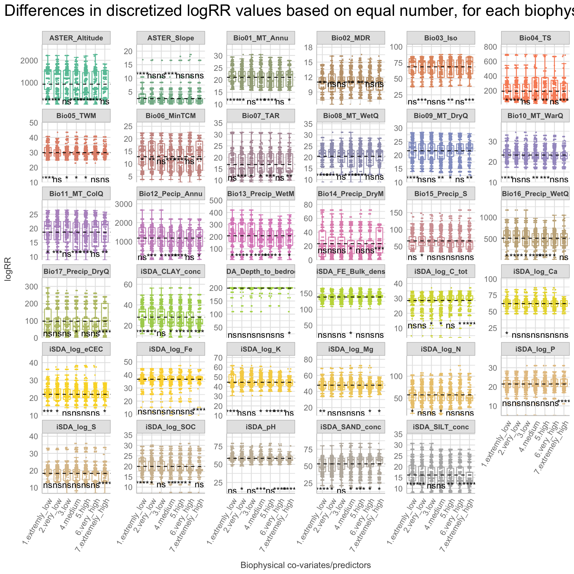
Figure 12: Boxplot of equal number discretized logRR vs. biophysical predictors
Correlation of features
We can use the the lares package is an R package built to automate, improve, and speed everyday analysis and machine learning tasks, build specifically for visualising regression and classification model performance by easily and intuitively giving most important plots, all generated at once. This function creates a correlation full study and returns a rank of the highest correlation variables obtained in a cross-table. Depending on input plot, we get correlation and p-value results for every combination of features, arranged by descending absolute correlation value.
Show code
agrofor.biophys.modelling.data.lares.corr <- readRDS(file = here::here("TidyMod_OUTPUT","agrofor.biophys.modelling.data.RDS"))
agrofor.biophys.modelling.data.lares.corr <-
agrofor.biophys.modelling.data.lares.corr %>%
dplyr::select(-c("RR", "ID", "AEZ16s", "Country", "MeanC", "MeanT", "PrName", "PrName.Code", "ID", "SubPrName", "Out.SubInd", "Product", "Product", "Country", "Site.Type", "Tree", "Out.SubInd.Code"))
# Show only most relevant results filtered by pvalue
lares::corr_cross(agrofor.biophys.modelling.data.lares.corr,
rm.na = TRUE,
max_pvalue = 0.05,
top = 20,
quiet = TRUE)
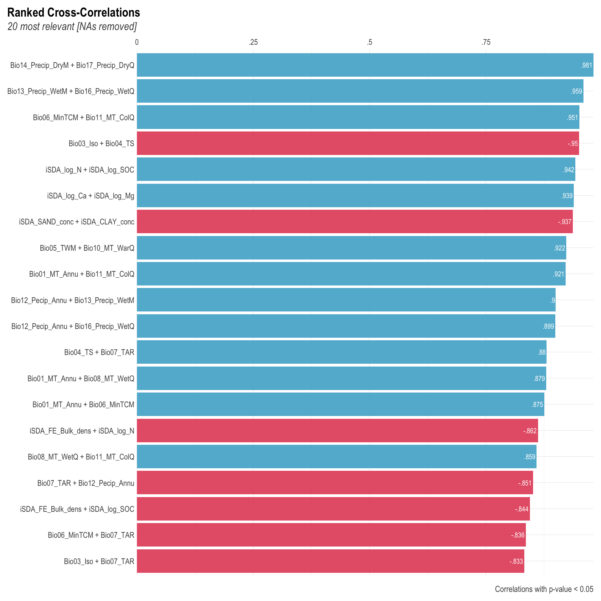
Figure 13: Ranked cross-correlation plot of numeric biophysical co-variables
There is another kind of cross-correlation that returns all correlations in a single plot, not necessarily ranked. This will help us understand the skewness or randomness of some correlations found. It will also highlight the highest correlations for each of the variables used.
Show code
# Cross-Correlation max values per category
lares::corr_cross(agrofor.biophys.modelling.data.lares.corr, type = 2, top = NA)
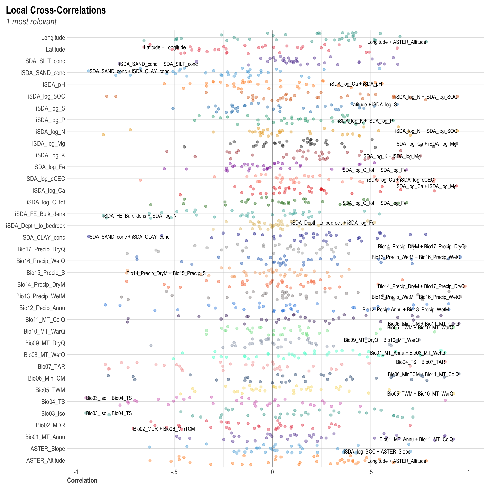
Figure 14: Ranked cross-correlation plot with all correlations of numeric biophysical co-variables
We are going to investigate the correlation among the continuous predictor features via the corrr package. This package is specifically designed to check for correlation between features. We are using the corrr::correlation() function to produce a correlation matrix with Pearson’s product-moment correlation coefficient. The correlation matrix is a measure of linear correlation between two variables in the agroforestry data. It is the ratio between the covariance of two variables and the product of their standard deviations; thus it essentially shows a normalised measurement of the covariance, between −1 (negatively correlated) and 1 (positively correlated). Hence, the coefficient indicates both the strength of the relationship as well as the direction. If two variables change in the same direction they are positively correlated. If the change in opposite directions together (one goes up, one goes down), then they are negatively correlated. As with covariance itself, the measure can only reflect a linear correlation of variables, and ignores many other types of relationship.
“Covariance” indicates the direction of the linear relationship between variables. “Correlation” on the other hand measures both the strength and direction of the linear relationship between two variables. Correlation is a function of the covariance. What sets them apart is the fact that correlation values are standardized whereas, covariance values are not.
Creating a correlation matrix is a useful step in our explanatory data analysis of our agroforestry data, because some machine learning algorithms like linear and logistic regression can have poor performance if there are highly correlated input variables in your data.
Lets first prepare a correlation matrix, that we can plot on a graph
agroforest.corr.cont.pred <- agrofor.biophys.modelling.data.numeric %>%
dplyr::select(Bio01_MT_Annu:ASTER_Slope) %>% # selecting predictor columns numeric data from the agrofor.biophys.modelling.data.numeric dataset
corrr::correlate() %>% # using the correlation() function to create the correlation matrix
corrr::focus(Bio01_MT_Annu:ASTER_Slope, mirror = TRUE) %>%
corrr::rearrange() # rearrange by correlations
# Using corrr::fashion() to print correlation matrix in a nicer format
# corrr::fashion(agroforest.corr.cont.pred)
# Correlation method: 'pearson'
# Missing treated using: 'pairwise.complete.obs'
#
# Registered S3 methods overwritten by 'registry':
# method from
# print.registry_field proxy
# print.registry_entry proxy
# SAVING CORR DATA
saveRDS(agroforest.corr.cont.pred, here::here("TidyMod_OUTPUT", "agroforest.corr.cont.pred.RDS"))
Correlation table
Show code
agroforest.corr.cont.pred <- readRDS( here::here("TidyMod_OUTPUT","agroforest.corr.cont.pred.RDS"))
rmarkdown::paged_table(agroforest.corr.cont.pred %>% shave() %>% corrr::fashion()) # shave off the upper triangle for a clean result
Now we can plot the correlation matrix visually interpret our correlation analysis
agroforest.corr.cont.pred.plot <- agroforest.corr.cont.pred %>%
shave() %>%
corrr::rplot(colours = c("#C6B18B","white","#66C2A5")) +
labs(title = "Correlation between biophysical predictors",
subtitle = "Pearson's correlation - for all ERA agroforestry practices with crop and biomass yield outcomes") +
expand_limits(x = c(-0.2, 0.2), y = c(-0.2, 0.2)) +
theme_lucid(plot.title.size = 25,
axis.title.size = 20,
axis.text.angle = 45,
legend.position = "right",
tags.size = 20,
legend.text.size = 15)
# SAVING CORR PLOT
saveRDS(agroforest.corr.cont.pred.plot, here::here("TidyMod_OUTPUT", "agroforest.corr.cont.pred.plot.RDS"))
Show code
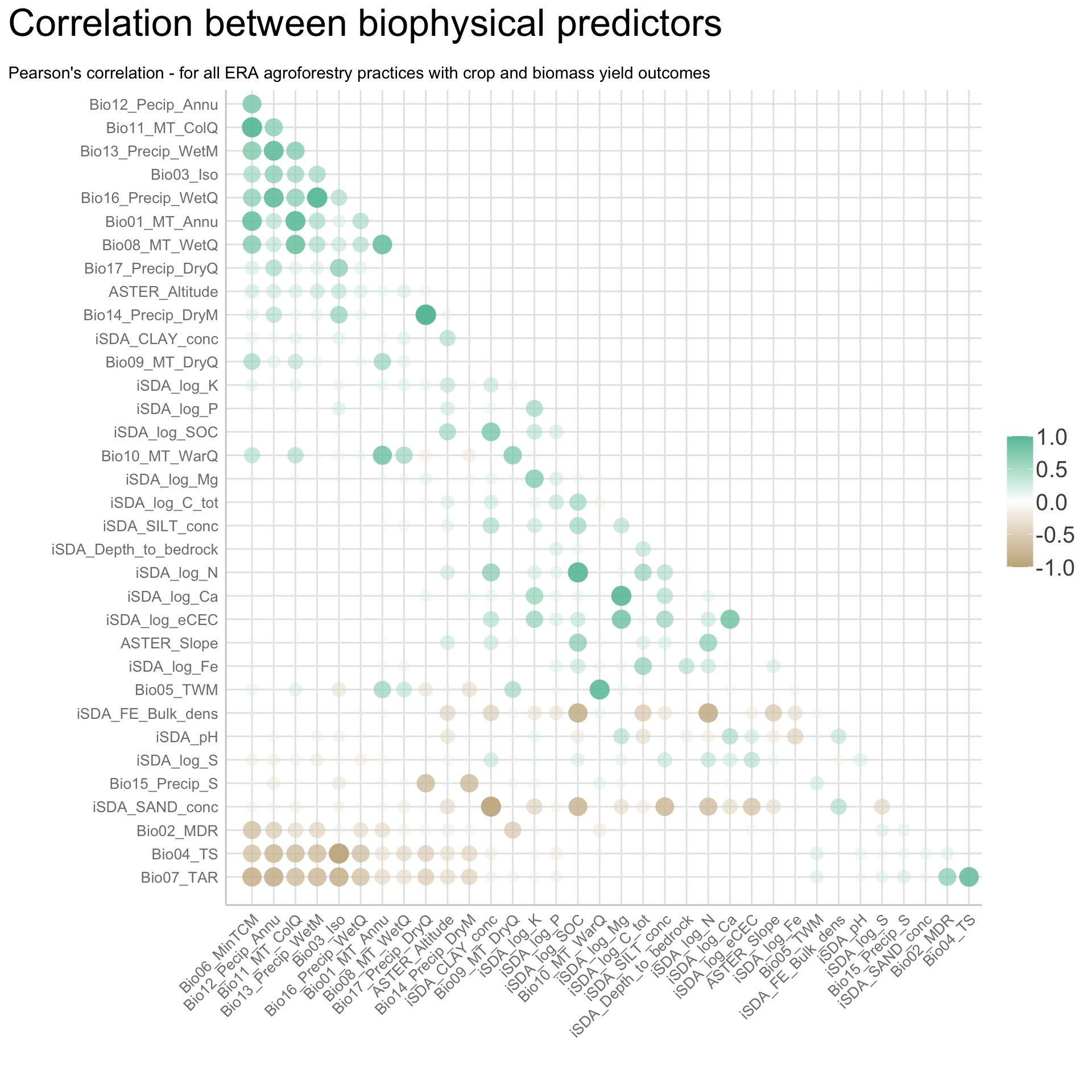
Figure 15: Correlation matrix plot of all biophysical predictors
Lets have a closer look at the correlation between RR and some of the numeric predictors by plotting another correlation matrix where we include logRR and filter rows to occasions in which logRR has a correlation of 0.7 or more with another variable.
agroforest.corr.cont.pred.logRR <- agrofor.biophys.modelling.data.numeric %>%
dplyr::select(logRR:ASTER_Slope) %>%
rationalize() %>%
drop_na() %>%
dplyr::select(logRR:ASTER_Slope) %>% # selecting logRR and predictor columns numeric data from the agrofor.biophys.modelling.data.numeric dataset
corrr::correlate() %>% # using the correlation() function to create the correlation matrix
focus(logRR:ASTER_Slope, mirror = TRUE) %>%
rearrange() # rearrange by correlations
# Correlation method: 'pearson'
# Missing treated using: 'pairwise.complete.obs'
agroforest.corr.cont.pred.logRR.plot <- agroforest.corr.cont.pred.logRR %>%
shave() %>%
corrr::rplot(colours = c("#C6B18B","white","#66C2A5")) +
labs(title = "Correlation between biophysical predictors and logRR",
subtitle = "Pearson's correlation - for all ERA agroforestry practices with crop and biomass yield outcomes") +
expand_limits(x = c(-0.2, 0.2), y = c(-0.2, 0.2)) +
theme_lucid(plot.title.size = 25,
axis.title.size = 20,
axis.text.angle = 45,
legend.position = "right",
tags.size = 20,
legend.text.size = 15)
# SAVING CORR PLOT
saveRDS(agroforest.corr.cont.pred.logRR.plot, here::here("TidyMod_OUTPUT", "agroforest.corr.cont.pred.logRR.plot.RDS"))
Lets plot the correlation matrix in which we have inclueded logRR
Show code
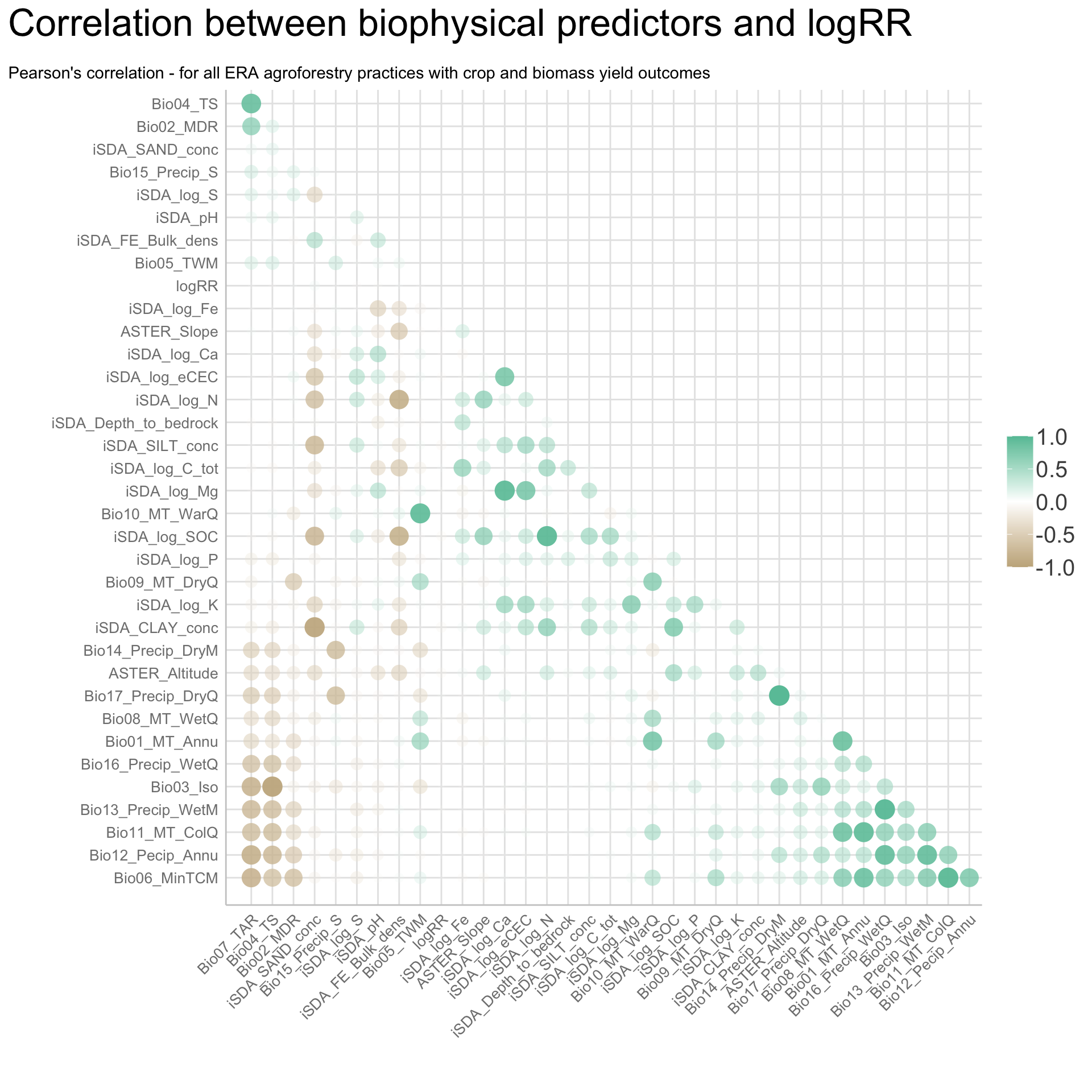
Figure 16: Correlation between biophysical predictors and logRR
agroforest.corr.cont.pred.logRR.results.filtered <- agroforest.corr.cont.pred.logRR %>%
filter(logRR > 0.019) %>%
relocate(term, logRR) %>%
arrange(desc(logRR))
# SAVING CORR DATA
saveRDS(agroforest.corr.cont.pred.logRR.results.filtered, here::here("TidyMod_OUTPUT", "agroforest.corr.cont.pred.logRR.results.filtered.RDS"))
Show code
agroforest.corr.cont.pred.logRR.results.filtered <- readRDS( here::here("TidyMod_OUTPUT","agroforest.corr.cont.pred.logRR.results.filtered.RDS"))
rmarkdown::paged_table(agroforest.corr.cont.pred.logRR.results.filtered)
Another way of visually examine correlations in our data is through a so called network correlation plot. Again the corrr package comes in handy as it has a plot function called network_plot() specifically for network correlations.
Show code
agroforest.network.corr.cont.pred.plot <- agroforest.corr.cont.pred %>%
network_plot(min_cor = .2, repel = TRUE, colours = c("#C6B18B","white","#66C2A5"), legend = TRUE, curved = TRUE) +
labs(title = "Network correlation between biophysical predictors",
subtitle = "Pearson's correlation [min. correlation = 0.2] - for all ERA agroforestry practices with crop and biomass yield outcomes") +
expand_limits(x = c(-0.2, 0.2), y = c(-0.2, 0.2)) +
theme_lucid(plot.title.size = 25,
legend.position = "right",
tags.size = 5,
legend.text.size = 15)
# SAVING NETWORK CORR PLOT
saveRDS(agroforest.network.corr.cont.pred.plot, here::here("TidyMod_OUTPUT", "agroforest.network.corr.cont.pred.plot.RDS"))
Show code
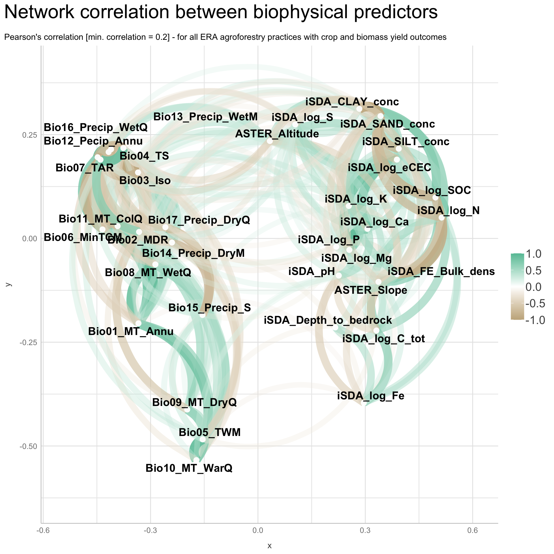
Figure 17: Network correlation plot between biophysical predictors and logRR
We see that there is clearly some of the biophysical predictor features that requires some serious attention to reduce the high correlation there is between some of them. Some features are obviously highly correlated, e.g. sand, clay and silts content, because they are expressed as percentage they are directly proportional to one another. For other features it is less obvious, e.g. clay and soil organic carbon or mean temperature of wettest month (Bio05_TWM) and mean temperature of warmest quarter (Bio10_MT_WarQ). Note that this correlation matrix only shows us linear relationships of features, and ignores other types of (more complex) relational patterns, that our machine learning algorithms might take advantage of.
Correlation between categorical variables
With colpair_map(), we have a way of comparing categorical columns with one another. Let’s try this with a few categorical columns from our agroforestry data
There are a few different ways of finding the strength of the relationship between two categorical variables. One useful measure is called Cramer’s V, which takes on values between 0 and 1 depending on how closely associated the variables are. Cramer’s V is used to examine the association between two categorical variables when there is more than a 2 X 2 contingency (e.g., 2 X 3)
Having the ability to use arbitrary functions like this opens up intriguing possibilities for analyzing data. One limitation of using only correlations is they will only work for continuous features. It is clear that there a several of the predictors that have a strong correlation (either positive of negative) and we would have to deal with this in our preprocessing steps.
Show code
agroforest.categorical.cramerV <- agrofor.biophys.modelling.data %>%
dplyr::select(AEZ16s,
PrName,
#PrName.Code,
SubPrName,
Product,
Out.SubInd,
#Out.SubInd.Code,
Country,
Site.Type,
Tree) %>%
rationalize() %>%
drop_na() %>%
colpair_map(rcompanion::cramerV, digits = 2)
agroforest.categorical.cramerV.plot <- agroforest.categorical.cramerV %>%
shave() %>%
corrr::rplot(colours = c("#C6B18B","white","#66C2A5")) +
labs(title = "Correlation between categorical features",
subtitle = "Cramer's V correlation - for all ERA agroforestry practices with crop and biomass yield outcomes") +
expand_limits(x = c(-0.2, 0.2), y = c(-0.2, 0.2)) +
theme_lucid(plot.title.size = 25,
axis.title.size = 20,
axis.text.angle = 45,
legend.position = "right",
tags.size = 20,
legend.text.size = 15)
# SAVING CRAMERS V DATA AND PLOT
saveRDS(agroforest.categorical.cramerV, here::here("TidyMod_OUTPUT", "agroforest.categorical.cramerV.RDS"))
saveRDS(agroforest.categorical.cramerV.plot, here::here("TidyMod_OUTPUT", "agroforest.categorical.cramerV.plot.RDS"))
Cramer’s V for association/correlation between categorical features
Show code
agroforest.categorical.cramerV <- readRDS( here::here("TidyMod_OUTPUT","agroforest.categorical.cramerV.RDS"))
rmarkdown::paged_table(agroforest.categorical.cramerV)
Show code
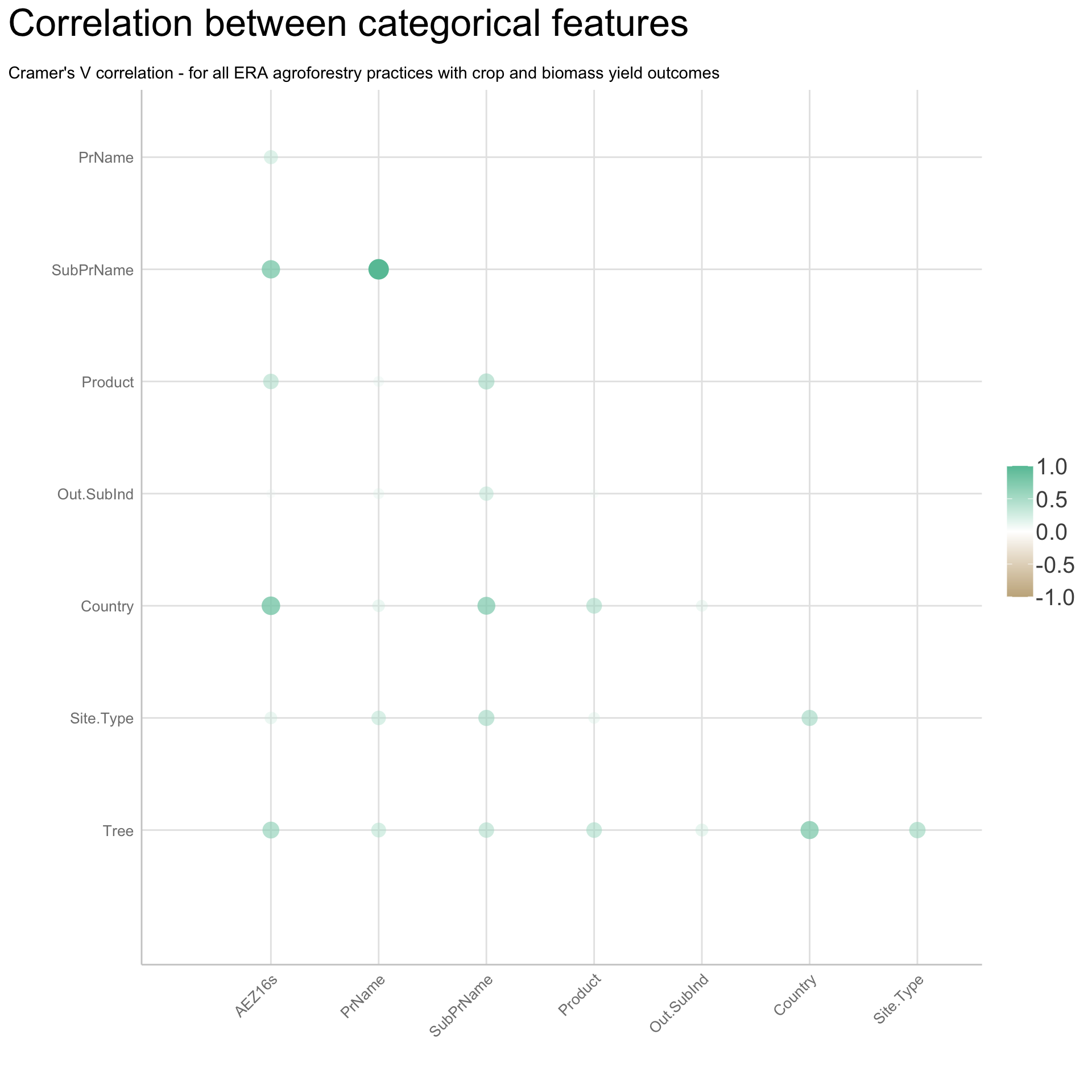
Figure 18: Cramers V correlation plot of selected catagorical variables
Scatter and Marginal Box and Density plots
With the combined use of scatter and marginal box or density plots we can get a good understanding of the the (linear) relationship between pairs of predictors and outcome (logRR). Lets have a look at the linear relationship between logRR and the biophysical predictor with the highest correlation coefficients, sand content () and total soil carbon (iSDA_log_C_tot). First we will make use of the wrapper package ggExtra, to create marginal density plots, and next use to package cowplot for generating scatter plots with marginal boxplots for multiple groups.
Scatter and density plot of total soil C and logRR
Show code
logRR_tot.soil.C <- ggscatter(agrofor.biophys.modelling.data, x = "iSDA_log_C_tot", y = "logRR",
alpha = 0, add = "reg.line", add.params = list(color = "#EBC97B"), conf.int = TRUE, cor.coef = TRUE, # adding confidence
cor.coeff.args = list(method = "pearson", label.x = -5, label.y = 2.8, label.sep = "\n")) + # correlation method
geom_jitter(size = 2, shape = 16, alpha = 0.1, width = 3, height = 0.5) + # adding jitter effect
labs(title = "Scatter and density plot of total soil C and logRR",
subtitle = "Scatter and marginal density plot with Pearson's correlation derived p-value and R coeffecient",
x = "Total soil organic carbon (log_C_tot)",
y = "Response ratio [log(RR)]")
scatter_density_totC_logRR <- ggExtra::ggMarginal(logRR_tot.soil.C, type = "density")
# SAVING PLOT
saveRDS(scatter_density_totC_logRR, here::here("TidyMod_OUTPUT", "scatter_density_totC_logRR.RDS"))
Scatter and density plot of sand content and logRR
Show code
logRR_sand.cont <- ggscatter(agrofor.biophys.modelling.data, x = "iSDA_SAND_conc", y = "logRR",
alpha = 0, add = "reg.line", add.params = list(color = "#EBC97B"), conf.int = TRUE, cor.coef = TRUE,
cor.coeff.args = list(method = "pearson", label.x = -5, label.y = 4, label.sep = "\n")) + # correlation method
geom_jitter(size = 2, shape = 16, alpha = 0.1, width = 3, height = 0.5) + # adding jitter effect
labs(title = "Scatter and density plot of sand content and logRR",
subtitle = "Scatter and marginal density plot with Pearson's correlation derived p-value and R coeffecient",
x = "Sand content [%]",
y = "Response ratio [log(RR)]")
scatter_density_sand_logRR <- ggExtra::ggMarginal(logRR_sand.cont, type = "density")
# SAVING PLOT
saveRDS(scatter_density_sand_logRR, here::here("TidyMod_OUTPUT", "scatter_density_sand_logRR.RDS"))
Scatter and density plot of Bio02 mean diurnal
\(temperature\) range (Bio02_MDR) and logRR
Show code
logRR_Bio02_MDR <- ggscatter(agrofor.biophys.modelling.data, x = "Bio02_MDR", y = "logRR",
alpha = 0, add = "reg.line", add.params = list(color = "#EBC97B"), conf.int = TRUE, cor.coef = TRUE,
cor.coeff.args = list(method = "pearson", label.x = 5, label.y = 4, label.sep = "\n")) + # correlation method
geom_jitter(size = 2, shape = 16, alpha = 0.1, width = 3, height = 0.5) + # adding jitter effect
labs(title = "Scatter and density plot of Bio02_MDR and logRR",
subtitle = "Scatter and marginal density plot with Pearson's correlation derived p-value and R coeffecient",
x = "Mean Diurnal Temperature Range",
y = "Response ratio [log(RR)]")
scatter_density_BIO.02_logRR <- ggExtra::ggMarginal(logRR_Bio02_MDR, type = "density")
# SAVING PLOT
saveRDS(scatter_density_BIO.02_logRR, here::here("TidyMod_OUTPUT", "scatter_density_BIO.02_logRR.RDS"))
The general relationship between logRR and these selected biphysical predictors is quite poor for all of these examples, even though they are the highest scoring predictors in the correlation matrix we did before. We just have to remain faithful that our machine learning algorithms can find more useful patterns in the collective set of predictors. One limitation of ggExtra package is that it can’t cope with multiple groups in the scatter plot and the marginal plots. Hence, bellow we are going to make use of the cowplot package. A package specifically designed as a simple add-on to ggplot. It provides various features that will help us with creating aligned plots awith multiple groups and arrange them in a neat way.
Lets make a cowplot with a scatter plot of logRR vs sand content and add two marginal plots = a boxplot that shows the differences between the outcomes crop and biomass yield and a density plot on the right side of the cowplot showing the well-known density distribution of the logRR response variable.
Ridge plots
This is interesting as we see how temperatures are distributed differently across agroforestry practices. Most noticably is that agroforestry parklands are generally represented in environments with higher temperatures. Contrary is that agroforestry noundary planting practices are mostly represented in environments that have lower temperatures.
BIO 1 - Mean Annual Temperature
Show code
dens.ridge.points.qq.bio1 <-
agrofor.biophys.modelling.data %>%
ggplot(aes(x = Bio01_MT_Annu, y = PrName, fill = ..x..)) +
geom_density_ridges_gradient(rel_min_height = 0,
jittered_points = TRUE,
position = position_points_jitter(width = 4, height = 0),
point_shape = '|',
point_size = 3,
point_alpha = 1,
quantile_lines = TRUE,
scale = 0.9,
alpha = 0.7,
vline_size = 1,
vline_color = "red") +
theme_lucid(plot.title.size = 25) +
theme(legend.position = "none",
panel.spacing = unit(0.2, "lines"),
strip.text.x = element_text(size = 8)) +
labs(title = "BIO.1 - Mean Annual Temperature distribution for all agroforestry practices with crop and biomass yield outcomes",
x = "BIO 1 - Mean Annual Temperature",
y = "ERA Agroforestry practice") +
scale_fill_viridis(option = "D")
# SAVING PLOT
saveRDS(dens.ridge.points.qq.bio1, here::here("TidyMod_OUTPUT", "dens.ridge.points.qq.bio1.RDS"))
Show code
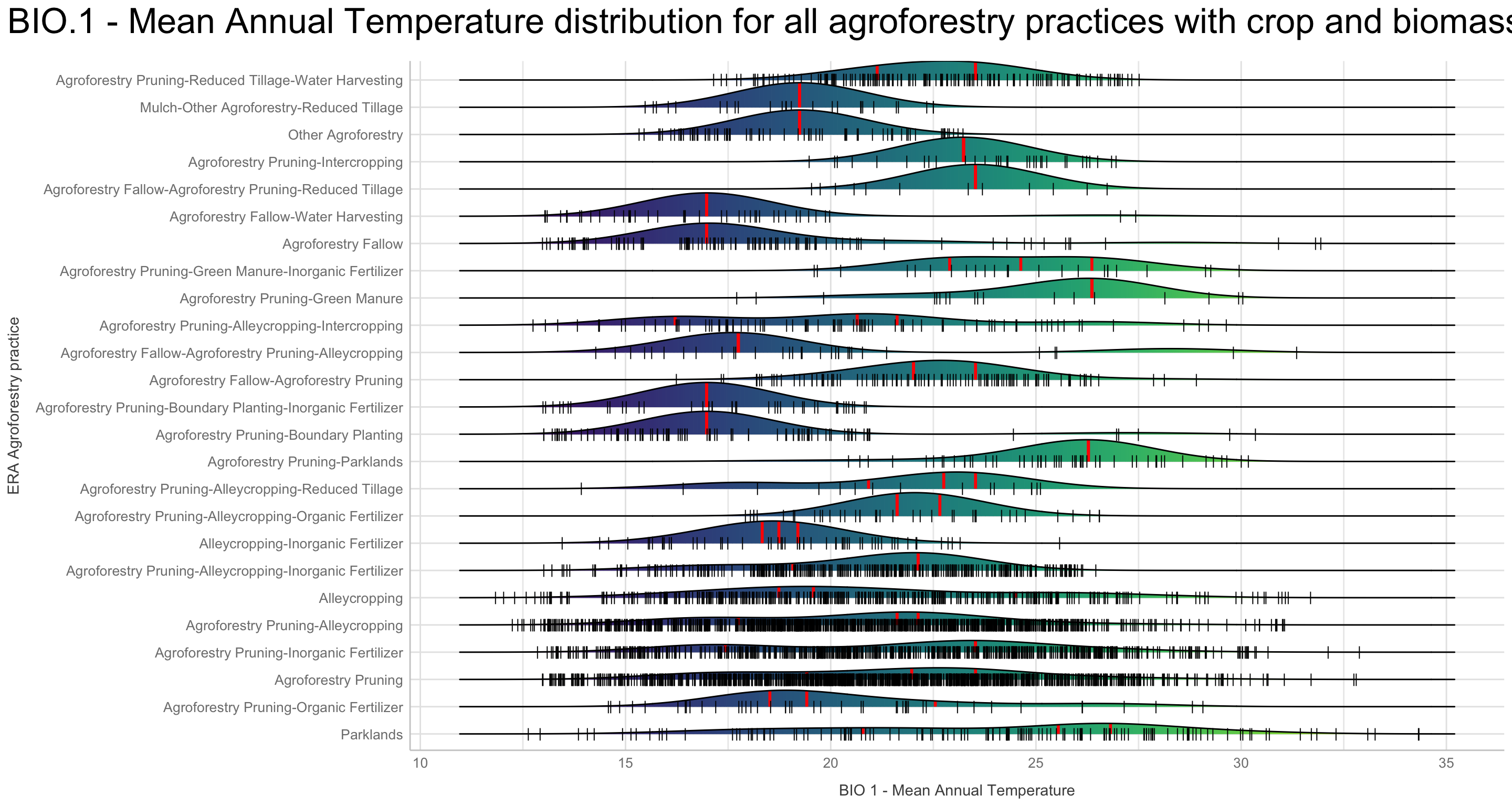
Figure 19: Density ridge plot for BIO.01 Mean Annual Temperature distribution across all agroforestry practices
Soil Organic Carbon
Show code
dens.ridge.points.qq.soilC <-
agrofor.biophys.modelling.data %>%
ggplot(aes(x = iSDA_log_SOC, y = PrName, fill = ..x..)) +
geom_density_ridges_gradient(rel_min_height = 0,
jittered_points = TRUE,
position = position_points_jitter(width = 4, height = 0),
point_shape = '|',
point_size = 3,
point_alpha = 1,
quantile_lines = TRUE,
scale = 0.9,
alpha = 0.7,
vline_size = 1,
vline_color = "red") +
theme_lucid(plot.title.size = 25) +
theme(legend.position = "none",
panel.spacing = unit(0.2, "lines"),
strip.text.x = element_text(size = 8)) +
labs(title = "Soil organic carbon distribution for all agroforestry practices with crop and biomass yield outcomes",
x = "log SOC",
y = "ERA Agroforestry practice") +
scale_fill_viridis(option = "D")
# SAVING PLOT
saveRDS(dens.ridge.points.qq.soilC, here::here("TidyMod_OUTPUT", "dens.ridge.points.qq.soilC.RDS"))
Show code
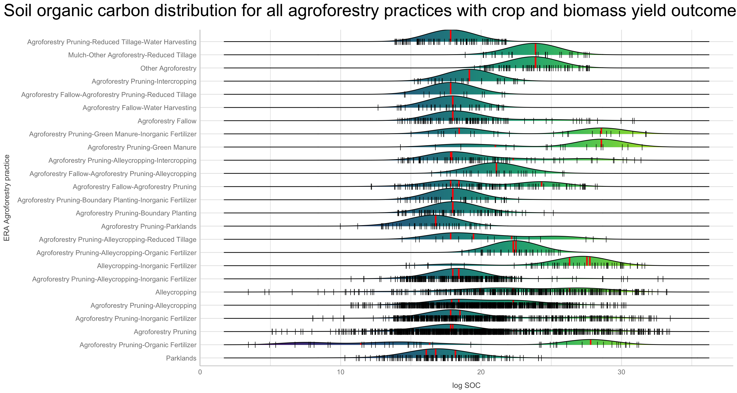
Figure 20: Density ridge plot forsoil organic carbon distribution across all agroforestry practices
Sand content
Show code
dens.ridge.points.qq.sand <-
agrofor.biophys.modelling.data %>%
ggplot(aes(x = iSDA_SAND_conc, y = PrName, fill = ..x..)) +
geom_density_ridges_gradient(rel_min_height = 0,
jittered_points = TRUE,
position = position_points_jitter(width = 4, height = 0),
point_shape = '|',
point_size = 3,
point_alpha = 1,
quantile_lines = TRUE,
scale = 0.9,
alpha = 0.7,
vline_size = 1,
vline_color = "red") +
theme_lucid(plot.title.size = 25) +
theme(legend.position = "none",
panel.spacing = unit(0.2, "lines"),
strip.text.x = element_text(size = 8)) +
labs(title = "Soil organic carbon distribution for all agroforestry practices with crop and biomass yield outcomes",
x = "Sand content",
y = "ERA Agroforestry practice") +
scale_fill_viridis(option = "D")
# SAVING PLOT
saveRDS(dens.ridge.points.qq.sand, here::here("TidyMod_OUTPUT", "dens.ridge.points.qq.sand.RDS"))
Show code
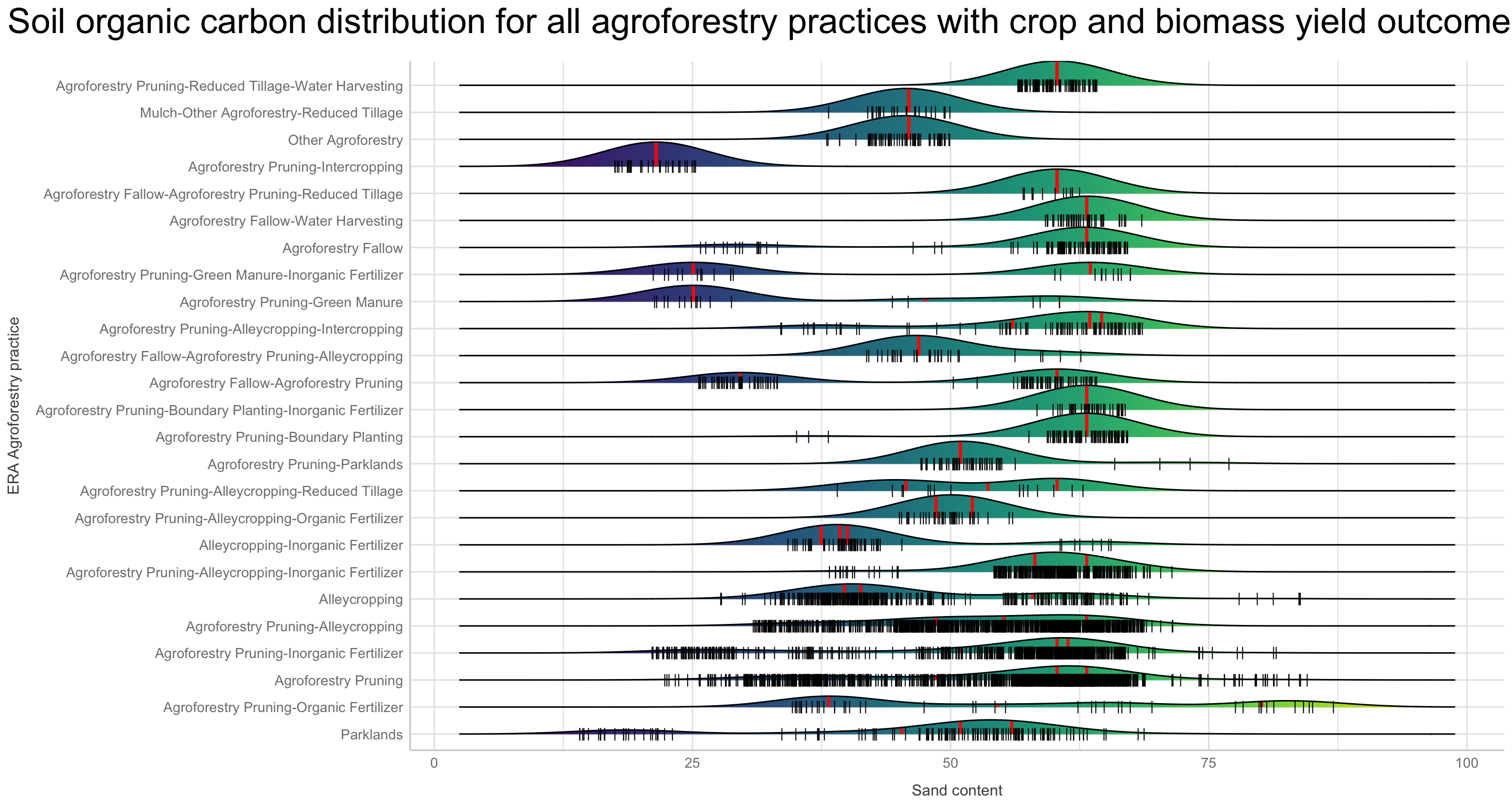
Figure 21: Density ridge plot for sand content distribution across all agroforestry practices
Could also be interesting to see how the sand content feature is distributet among the discritized logRR groups
For the equal number discritization
Show code
dens.ridge.EQNo.discritized.logRR.sand <-
par.coord.data.EQNo %>%
ggplot(aes(x = iSDA_SAND_conc, y = logRR_EQNo_group, fill = ..x..)) +
geom_density_ridges_gradient(rel_min_height = 0,
jittered_points = TRUE,
position = position_points_jitter(width = 4, height = 0),
point_shape = '|',
point_size = 3,
point_alpha = 1,
quantile_lines = TRUE,
scale = 0.9,
alpha = 0.7,
vline_size = 1,
vline_color = "red") +
theme_lucid(plot.title.size = 25) +
theme(legend.position = "none",
panel.spacing = unit(0.2, "lines"),
strip.text.x = element_text(size = 8)) +
labs(title = "Sand content distribution across the seven clases of EQNo discritized logRR groups",
x = "Sand content",
y = "Discretised groups of logRR") +
scale_fill_viridis(option = "D")
# SAVING PLOT
saveRDS(dens.ridge.EQNo.discritized.logRR.sand, here::here("TidyMod_OUTPUT", "dens.ridge.EQNo.discritized.logRR.sand.RDS"))
Show code
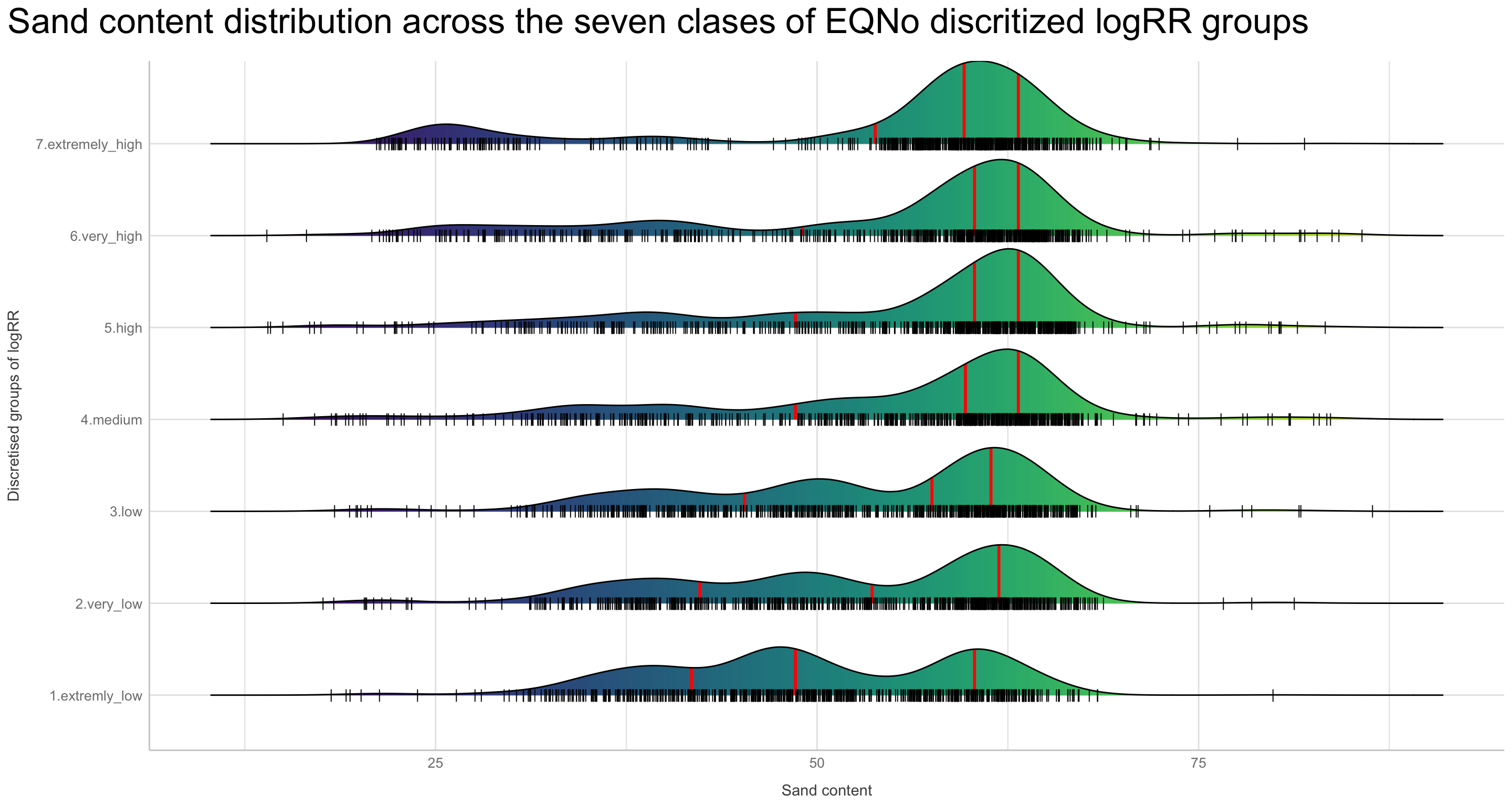
Figure 22: Density ridge plot for sand content distribution across the EQNo discritized logRR groupss
For the equal range discritization
Show code
dens.ridge.EQR.discritized.logRR.sand <-
agrofor.biophys.modelling.data.discretized.logRR %>%
ggplot(aes(x = iSDA_SAND_conc, y = logRR_EQR_group, fill = ..x..)) +
geom_density_ridges_gradient(rel_min_height = 0,
jittered_points = TRUE,
position = position_points_jitter(width = 4, height = 0),
point_shape = '|',
point_size = 3,
point_alpha = 1,
quantile_lines = TRUE,
scale = 0.9,
alpha = 0.7,
vline_size = 1,
vline_color = "red") +
theme_lucid(plot.title.size = 25) +
theme(legend.position = "none",
panel.spacing = unit(0.2, "lines"),
strip.text.x = element_text(size = 8)) +
labs(title = "Sand concentration distribution across the seven clases of EQR discritized logRR groups",
x = "Sand concentration",
y = "Discretised groups of logRR") +
scale_fill_viridis(option = "D")
# SAVING PLOT
saveRDS(dens.ridge.EQR.discritized.logRR.sand, here::here("TidyMod_OUTPUT", "dens.ridge.EQR.discritized.logRR.sand.RDS"))
Show code
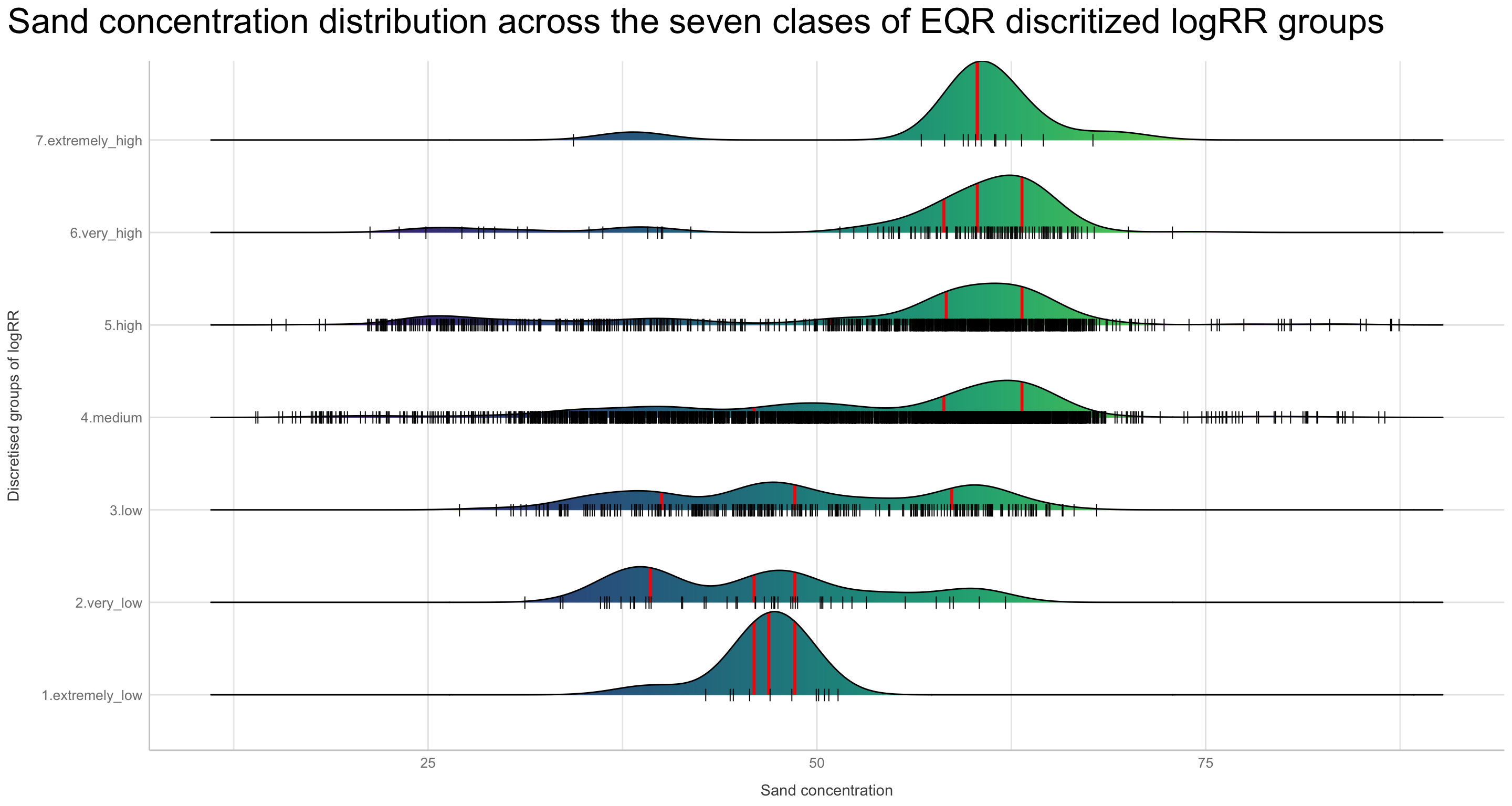
Figure 23: Density ridge plot for sand content distribution across the EQR discritized logRR groupss
Plotting logRR and selected biophysical predictors spatially
We hypothersise that the outcome feature, logRR, is assosiated with our biophysical predictors, but what about the spatial distribution of the logRR values. As the last step in our EDA, lets view the logRR and a group of selected biophysical predictors in a spatial dimension. We are going to use the coordinates (Longitude and Latitude) of the agroforestry data and use them to plot logRR on a hexaplot with colours of logRR values depending on whether they are high or low. First we will have to make am agroforestry dataset with no NA cells, as this is not meaningful.
How is the logRR values distributed on the continent..?
Show code
agrofor.biophys.modelling.data.raz <- agrofor.biophys.modelling.data %>%
rationalize() %>%
drop_na()
# SAVING DATA
saveRDS(agrofor.biophys.modelling.data.raz, here::here("TidyMod_OUTPUT", "agrofor.biophys.modelling.data.raz.RDS"))
logRR.plot <-
agrofor.biophys.modelling.data.raz %>%
select("logRR", "Longitude", "Latitude") %>%
ggplot(aes(Longitude, Latitude, z = logRR)) +
stat_summary_hex(alpha = 0.8, bins = 40) +
scale_fill_viridis_c(option = "magma") +
labs(
fill = "mean",
title = "logRR"
)
# SAVING NETWORK CORR PLOT
saveRDS(logRR.plot, here::here("TidyMod_OUTPUT", "logRR.plot.RDS"))
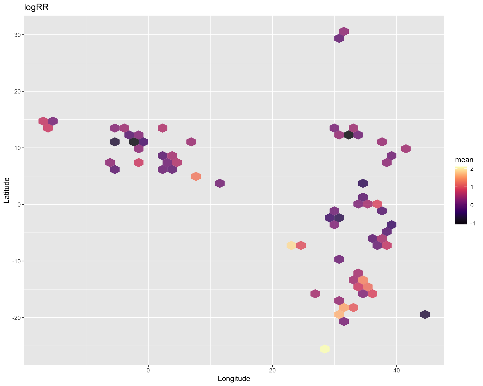
Figure 24: Spatial distribution of logRR values
Interesting! We do see an indication of spatially dependency of logRR values. Perhaps this is related to the agroecological climates in the locations? Unfortunately the spatial resolution is too course to actually open the possibility of conducting a proper in-depth spatial analysis.
Let us not look at the spatial variability for a number of selected biophysical predictors. We are going to create a little function that we call “pred.spatial.” We can apply this function on any of the agroforestry predictor features. The function will only require the coordinates (Longitude and Latitude) and a variable of interest.
agrofor.biophys.modelling.data.raz <- readRDS( here::here("TidyMod_OUTPUT","agrofor.biophys.modelling.data.raz.RDS"))
pred.spatial <- function(var, title) {
agrofor.biophys.modelling.data.raz %>%
ggplot(aes(Longitude, Latitude, z = {{ var }})) +
stat_summary_hex(alpha = 0.8, bins = 40) +
scale_fill_viridis_c(option = "magma") +
labs(
fill = "mean",
title = title
)
}
We are now going to use the function to look at a set of selected biophysical predictors and align them in a 3 x 3 multiples plot using the patchwork package, designed to make it simple and very intuitive to quickly combine separate ggplots into the same graphic.
Show code
(logRR.plot + pred.spatial(Bio01_MT_Annu, "BIO.01 - Mean Annual Temperature") + pred.spatial(Bio03_Iso, "BIO.03 - Isothermality")) /
(pred.spatial(Bio07_TAR, "BIO.07 - Annual Temperature Range") + pred.spatial(Bio12_Pecip_Annu, "BIO.12 - Annual Precipitation") + pred.spatial(Bio17_Precip_DryQ, "BIO.17 - Precipitation of Driest Quarter")) /
(pred.spatial(iSDA_SAND_conc, "Sand concentration") + pred.spatial(iSDA_log_C_tot, "Total soil carbon") + pred.spatial(iSDA_pH, "pH"))
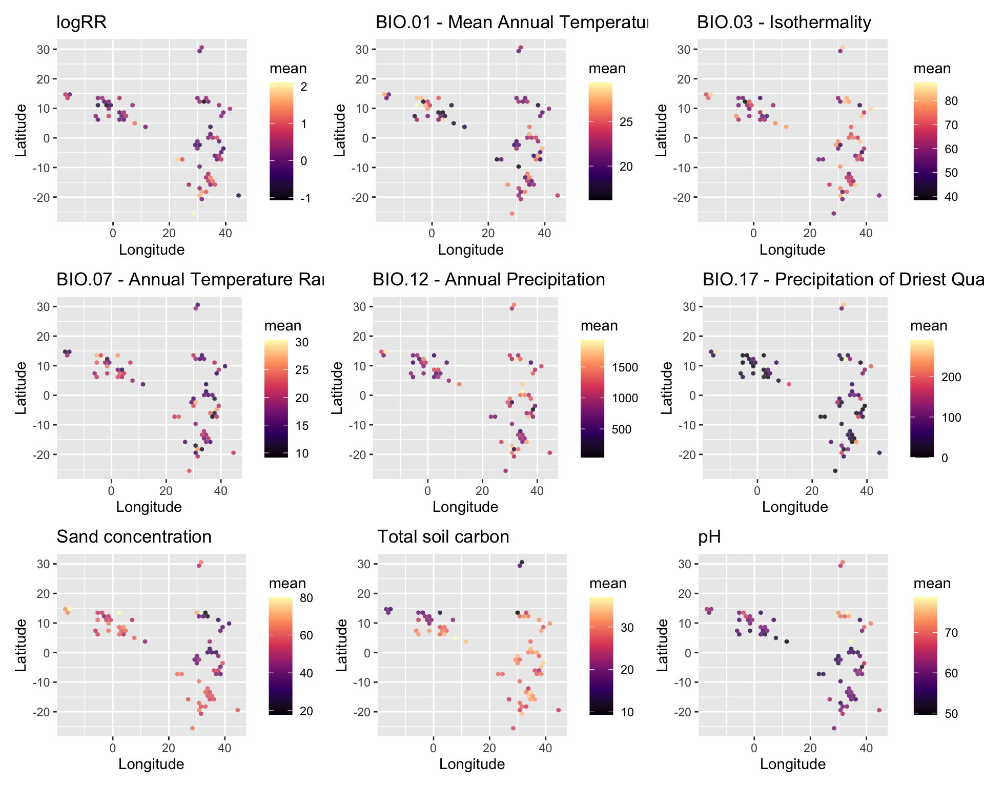
Figure 25: Spatial distribution of selected biophysical predictors
Boruta: Wrapper Algorithm for All Relevant Feature Selection
Boruta is an all relevant feature selection wrapper algorithm. It finds relevant features by comparing original attributes’ importance with importance achievable at random, estimated using their permuted copies (shadows). It is an all relevant feature selection method, while most other are minimal optimal; this means it tries to find all features carrying information usable for prediction, rather than finding a possibly compact subset of features on which some classifier has a minimal error.
Boruta iteratively compares importances of attributes with importances of shadow attributes, created by shuffling original ones. Attributes that have significantly worst importance than shadow ones are being consecutively dropped. On the other hand, attributes that are significantly better than shadows are admitted to be Confirmed. Shadows are re-created in each iteration. Algorithm stops when only Confirmed attributes are left, or when it reaches maxRuns importance source runs. If the second scenario occurs, some attributes may be left without a decision. They are claimed Tentative. You may try to extend maxRuns or lower pValue to clarify them, but in some cases their importances do fluctuate too much for Boruta to converge. Instead, you can use TentativeRoughFix function, which will perform other, weaker test to make a final decision, or simply treat them as undecided in further analysis. It is actually pretty trivial, no magic at all. The core idea is that a feature that is not relevant is not more useful for classification than its version with a permuted order of values. To this end, Boruta extends the given dataset with such permuted copies of all features (which we call shadows), applies some feature importance measure (aka VIM; Boruta can use any, the default is Random Forest’s MDA) and checks which features are better and which are worse than a most important shadow. The next important idea is based on observation that VIMs get more accurate with less irrelevant features present; thus, Boruta applies the above test iteratively, constantly removing features which it strongly believes are irrelevant.
In Boruta, features do not compete among themselves. Instead - and this is the first brilliant idea - they compete with a randomized version of themselves.
Show code
agrofor.boruta.with.tree <- as.data.table(data.table::copy(agrofor.biophys.modelling.data)) %>%
dplyr::select(-c(MeanC, # Outcome variable(s)
MeanT,
RR,
ID, # ID variable (will not be included as predictor)
AEZ16s, # ID variable (will not be included as predictor)
PrName, # ID variable (will not be included as predictor)
PrName.Code, # ID variable (will not be included as predictor)
SubPrName, # ID variable (will not be included as predictor)
Product, # ID variable (will not be included as predictor)
Out.SubInd, # ID variable (will not be included as predictor)
Out.SubInd.Code, # ID variable (will not be included as predictor)
Country, # ID variable (will not be included as predictor)
Latitude, # ID variable (will not be included as predictor, but as a basis for the spatial/cluster cross-validation)
Longitude, # ID variable (will not be included as predictor, but as a basis for the spatial/cluster cross-validation)
#Site.Type, # Site_Type will be included as predictor, to see how much it explains the outcome
#Tree # Tree will be included as predictor, to see how much it explains the outcome
)
) %>%
rationalize() %>%
drop_na()
# distinct(PrName, .keep_all = TRUE)
set.seed(1407)
agrofor.boruta.with.tree <- Boruta::Boruta(logRR ~ ., data = agrofor.boruta.with.tree,
pValue = 0.01,
mcAdj = TRUE,
holdHistory = TRUE,
doTrace = 3,
maxRuns = 200,
getImp = getImpRfZ)
# --------------------------------------------------------------------------------------------------------------------------------------------------------
# agrofor.boruta.with.tree
# Boruta performed 16 iterations in 1.193105 mins.
# 37 attributes confirmed important: ASTER_Altitude, ASTER_Slope, Bio01_MT_Annu, Bio02_MDR, Bio03_Iso and 32 more;
# No attributes deemed unimportant.
# SAVING DATA
saveRDS(agrofor.boruta.with.tree, here::here("TidyMod_OUTPUT", "agrofor.boruta.with.tree.RDS"))
Show code
agrofor.boruta.without.tree <- as.data.table(data.table::copy(agrofor.biophys.modelling.data)) %>%
dplyr::select(-c(MeanC, # Outcome variable(s)
MeanT,
RR,
ID, # ID variable (will not be included as predictor)
AEZ16s, # ID variable (will not be included as predictor)
PrName, # ID variable (will not be included as predictor)
PrName.Code, # ID variable (will not be included as predictor)
SubPrName, # ID variable (will not be included as predictor)
Product, # ID variable (will not be included as predictor)
Out.SubInd, # ID variable (will not be included as predictor)
Out.SubInd.Code, # ID variable (will not be included as predictor)
Country, # ID variable (will not be included as predictor)
Tree, # The Tree feature is excluded
Latitude, # ID variable (will not be included as predictor, but as a basis for the spatial/cluster cross-validation)
Longitude, # ID variable (will not be included as predictor, but as a basis for the spatial/cluster cross-validation)
#Site.Type, # Site_Type will be included as predictor, to see how much it explains the outcome
#Tree # Tree will be included as predictor, to see how much it explains the outcome
)
) %>%
rationalize() %>%
drop_na()
# distinct(PrName, .keep_all = TRUE)
set.seed(1407)
agrofor.boruta.without.tree <- Boruta::Boruta(logRR ~ ., data = agrofor.boruta.without.tree,
pValue = 0.01,
mcAdj = TRUE,
holdHistory = TRUE,
doTrace = 3,
maxRuns = 200,
getImp = getImpRfZ)
# --------------------------------------------------------------------------------------------------------------------------------------------------------
# agrofor.boruta.without.tree
# Boruta performed 20 iterations in 1.329663 mins.
# 36 attributes confirmed important: ASTER_Altitude, ASTER_Slope, Bio01_MT_Annu, Bio02_MDR, Bio03_Iso and 31 more;
# No attributes deemed unimportant.
# SAVING DATA
saveRDS(agrofor.boruta.without.tree, here::here("TidyMod_OUTPUT", "agrofor.boruta.without.tree.RDS"))
“What is to be sought in designs for the display of information is the clear portrayal of complexity. Not the complication of the simple; rather … the revelation of the complex.”
Show code
# LOADING BORUTA RESULTS --------------------------------------------------------------------------------
agrofor.boruta.with.tree <- readRDS( here::here("TidyMod_OUTPUT","agrofor.boruta.with.tree.RDS"))
plot(agrofor.boruta.with.tree, xlab = "", xaxt = "n")
lz <- lapply(1:ncol(agrofor.boruta.with.tree$ImpHistory),function(i)
agrofor.boruta.with.tree$ImpHistory[is.finite(agrofor.boruta.with.tree$ImpHistory[,i]),i])
names(lz) <- colnames(agrofor.boruta.with.tree$ImpHistory)
Labels <- sort(sapply(lz, median))
axis(side = 1, las = 2, labels = names(Labels), at = 1:ncol(agrofor.boruta.with.tree$ImpHistory), cex.axis = 0.5)
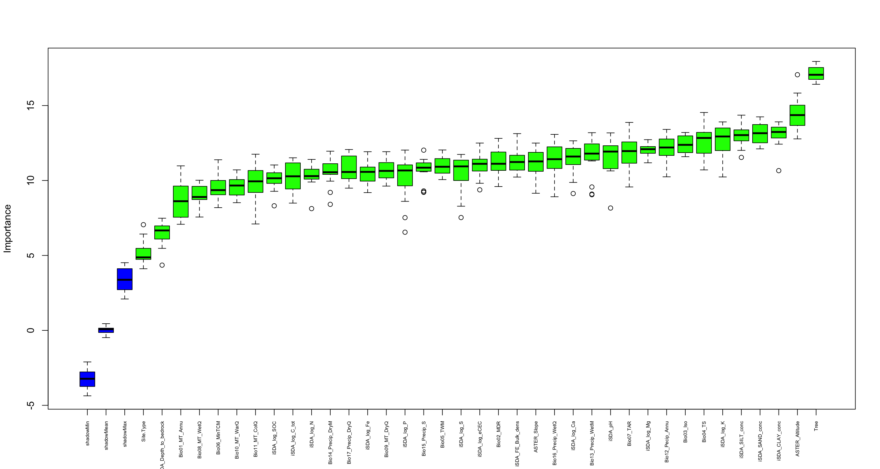
Figure 26: Boruta plot of biophysical predictors with the tree feature included
Show code
# LOADING BORUTA RESULTS --------------------------------------------------------------------------------
agrofor.boruta.without.tree <- readRDS( here::here("TidyMod_OUTPUT","agrofor.boruta.without.tree.RDS"))
plot(agrofor.boruta.without.tree, xlab = "", xaxt = "n")
lz <- lapply(1:ncol(agrofor.boruta.without.tree$ImpHistory),function(i)
agrofor.boruta.without.tree$ImpHistory[is.finite(agrofor.boruta.without.tree$ImpHistory[,i]),i])
names(lz) <- colnames(agrofor.boruta.without.tree$ImpHistory)
Labels <- sort(sapply(lz, median))
axis(side = 1, las = 2, labels = names(Labels), at = 1:ncol(agrofor.boruta.without.tree$ImpHistory), cex.axis = 0.5)
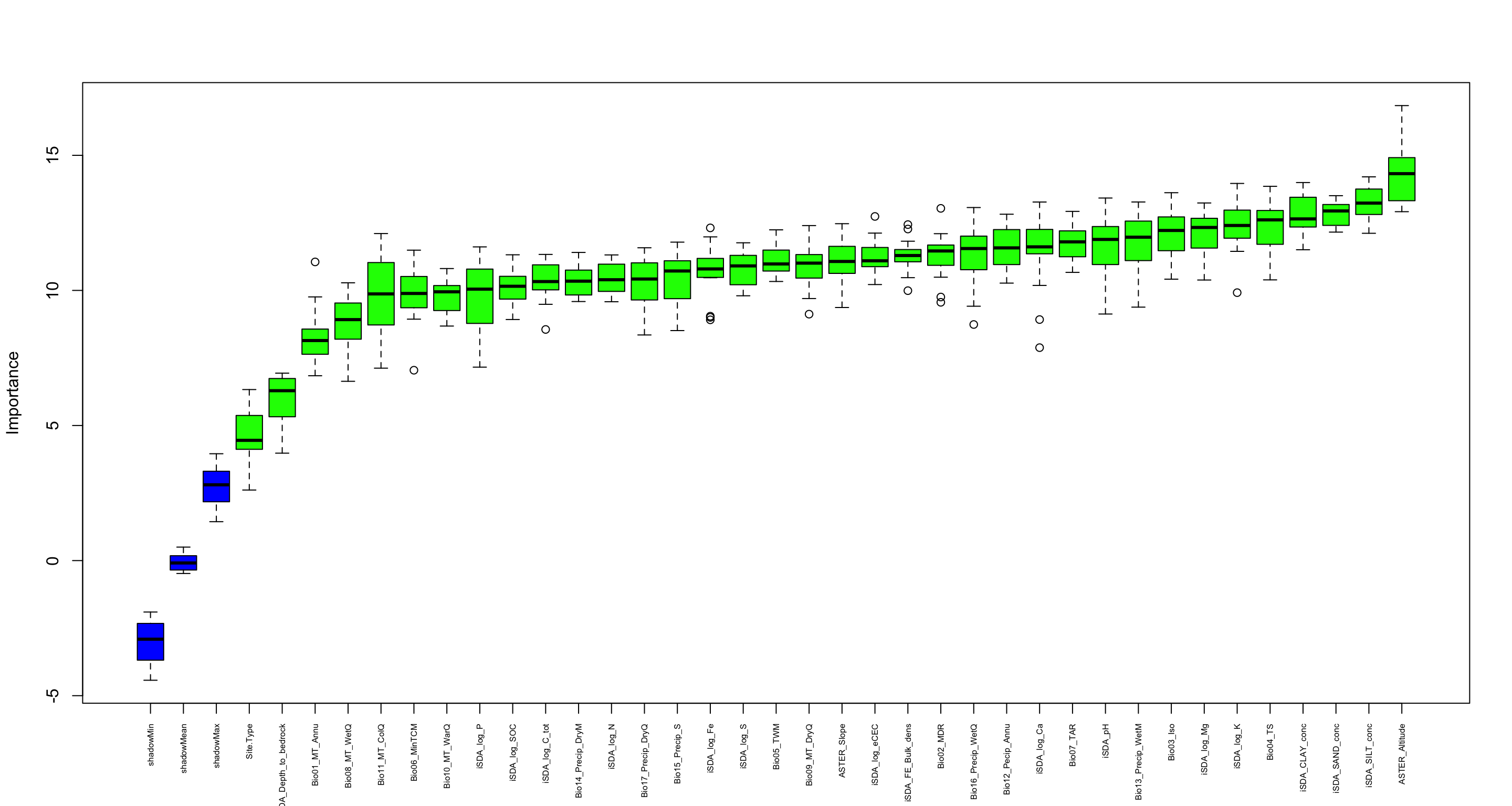
Figure 27: Boruta plot of biophysical predictors with the tree feature excluded
This plot reveals the importance of each of the features/attributes. There were no tentative attributes after the Boruta analysis for neither of the cases. Normally this is where it is the time to take decision on tentative attributes. The tentative attributes can be classified as confirmed or rejected by comparing the median Z score of the attributes with the median Z score of the best shadow attribute. However this is not nessesary now as all variables were confirmed to be important.
The columns in green are ‘confirmed’ and the ones in red are not. There are couple of blue bars representing ShadowMax and ShadowMin. They are not actual features, but are used by the boruta algorithm to decide if a variable is important or not.
Note: the code below shows how the final boruta analysis can be obtained
Show code
# --------------------------------------------------------------------------------------------------------------------------------------------------------
# agrofor.boruta.with.tree
agrofor.boruta.with.tree.final <- TentativeRoughFix(agrofor.boruta.with.tree)
print(agrofor.boruta.with.tree.final)
# Warning in TentativeRoughFix(agrofor.boruta.with.tree) :
# There are no Tentative attributes! Returning original object.
# Boruta performed 16 iterations in 2.665884 mins.
# 37 attributes confirmed important: ASTER_Altitude, ASTER_Slope, Bio01_MT_Annu, Bio02_MDR, Bio03_Iso and 32 more;
# No attributes deemed unimportant.
# --------------------------------------------------------------------------------------------------------------------------------------------------------
# agrofor.boruta.without.tree
agrofor.boruta.without.tree.final <- TentativeRoughFix(agrofor.boruta.without.tree)
print(agrofor.boruta.without.tree.final)
# Warning in TentativeRoughFix(agrofor.boruta.without.tree) :
# There are no Tentative attributes! Returning original object.
# Boruta performed 20 iterations in 1.329663 mins.
# 36 attributes confirmed important: ASTER_Altitude, ASTER_Slope, Bio01_MT_Annu, Bio02_MDR, Bio03_Iso and 31 more;
# No attributes deemed unimportant.
Listing the results of the Boruta analysis.
Show code
agrofor.boruta.with.tree.final.attribute.results <- getSelectedAttributes(agrofor.boruta.with.tree, withTentative = F)
agrofor.boruta.with.tree.final.attribute.results.df <- attStats(agrofor.boruta.with.tree)
agrofor.boruta.with.tree.final.attribute.results.df %>%
arrange(desc(meanImp))
meanImp medianImp minImp maxImp
Tree 17.141036 17.053639 16.418196 17.942156
ASTER_Altitude 14.444269 14.363125 12.776204 17.056516
iSDA_SAND_conc 13.181425 13.154695 12.110366 14.246089
iSDA_CLAY_conc 13.092710 13.236354 10.657800 13.911669
iSDA_SILT_conc 13.015519 13.028392 11.540338 14.358846
iSDA_log_K 12.712861 12.935984 10.236629 13.908092
Bio04_TS 12.629943 12.837434 10.707060 14.537330
Bio03_Iso 12.410692 12.378416 11.587653 13.202462
Bio12_Pecip_Annu 12.132579 12.200923 10.245201 13.408135
iSDA_log_Mg 12.009092 12.088222 11.180053 12.724573
Bio07_TAR 11.906894 11.961897 9.569568 13.874477
iSDA_pH 11.576551 11.928807 8.162786 13.176533
Bio13_Precip_WetM 11.540850 11.794833 9.051393 13.189559
iSDA_log_Ca 11.419733 11.599025 9.130097 12.646765
Bio16_Precip_WetQ 11.332354 11.421499 8.915385 13.075725
iSDA_FE_Bulk_dens 11.331999 11.232778 10.228500 13.127609
Bio02_MDR 11.286406 11.115773 9.595821 12.810161
ASTER_Slope 11.192857 11.272956 9.148335 12.496574
iSDA_log_eCEC 11.000078 11.112414 9.376787 12.497559
Bio05_TWM 10.986136 10.916895 10.059021 12.036749
Bio17_Precip_DryQ 10.771829 10.567620 9.488403 12.065971
Bio09_MT_DryQ 10.709578 10.639968 9.626701 11.921926
Bio15_Precip_S 10.708338 10.854826 9.211757 12.023778
Bio14_Precip_DryM 10.568750 10.550956 8.408274 11.954372
iSDA_log_S 10.521807 10.940608 7.528624 11.739296
iSDA_log_Fe 10.464748 10.574887 9.191623 11.920558
iSDA_log_N 10.327706 10.292425 8.124063 11.406045
iSDA_log_C_tot 10.249609 10.279400 8.490582 11.514404
iSDA_log_P 10.141530 10.668541 6.549487 12.029235
iSDA_log_SOC 10.084520 10.148419 8.311810 11.035104
Bio11_MT_ColQ 9.885578 9.943642 7.099605 11.753388
Bio10_MT_WarQ 9.621432 9.664511 8.519339 10.708570
Bio06_MinTCM 9.531914 9.357811 8.188499 11.382789
Bio08_MT_WetQ 9.031193 8.898862 7.563226 10.015798
Bio01_MT_Annu 8.728339 8.617663 7.078522 10.976606
iSDA_Depth_to_bedrock 6.428382 6.667476 4.352349 7.483126
Site.Type 5.148939 4.870930 4.111326 7.050893
normHits decision
Tree 1.0000 Confirmed
ASTER_Altitude 1.0000 Confirmed
iSDA_SAND_conc 1.0000 Confirmed
iSDA_CLAY_conc 1.0000 Confirmed
iSDA_SILT_conc 1.0000 Confirmed
iSDA_log_K 1.0000 Confirmed
Bio04_TS 1.0000 Confirmed
Bio03_Iso 1.0000 Confirmed
Bio12_Pecip_Annu 1.0000 Confirmed
iSDA_log_Mg 1.0000 Confirmed
Bio07_TAR 1.0000 Confirmed
iSDA_pH 1.0000 Confirmed
Bio13_Precip_WetM 1.0000 Confirmed
iSDA_log_Ca 1.0000 Confirmed
Bio16_Precip_WetQ 1.0000 Confirmed
iSDA_FE_Bulk_dens 1.0000 Confirmed
Bio02_MDR 1.0000 Confirmed
ASTER_Slope 1.0000 Confirmed
iSDA_log_eCEC 1.0000 Confirmed
Bio05_TWM 1.0000 Confirmed
Bio17_Precip_DryQ 1.0000 Confirmed
Bio09_MT_DryQ 1.0000 Confirmed
Bio15_Precip_S 1.0000 Confirmed
Bio14_Precip_DryM 1.0000 Confirmed
iSDA_log_S 1.0000 Confirmed
iSDA_log_Fe 1.0000 Confirmed
iSDA_log_N 1.0000 Confirmed
iSDA_log_C_tot 1.0000 Confirmed
iSDA_log_P 1.0000 Confirmed
iSDA_log_SOC 1.0000 Confirmed
Bio11_MT_ColQ 1.0000 Confirmed
Bio10_MT_WarQ 1.0000 Confirmed
Bio06_MinTCM 1.0000 Confirmed
Bio08_MT_WetQ 1.0000 Confirmed
Bio01_MT_Annu 1.0000 Confirmed
iSDA_Depth_to_bedrock 0.9375 Confirmed
Site.Type 1.0000 ConfirmedShow code
agrofor.boruta.without.tree.final.attribute.results <- getSelectedAttributes(agrofor.boruta.without.tree, withTentative = F)
agrofor.boruta.without.tree.final.attribute.results.df <- attStats(agrofor.boruta.without.tree)
agrofor.boruta.without.tree.final.attribute.results.df %>%
arrange(desc(meanImp))
meanImp medianImp minImp maxImp
ASTER_Altitude 14.327110 14.321245 12.913701 16.840116
iSDA_SILT_conc 13.241855 13.231626 12.114164 14.202938
iSDA_SAND_conc 12.860327 12.940649 12.157818 13.506262
iSDA_CLAY_conc 12.811644 12.646227 11.505049 13.992292
iSDA_log_K 12.421814 12.403131 9.917149 13.959016
Bio04_TS 12.368198 12.610442 10.389999 13.852030
iSDA_log_Mg 12.097006 12.329409 10.384763 13.236365
Bio03_Iso 12.066629 12.218784 10.415868 13.616036
Bio13_Precip_WetM 11.841693 11.969714 9.380817 13.272882
Bio07_TAR 11.768796 11.796537 10.667357 12.924934
iSDA_pH 11.696950 11.886987 9.126139 13.418997
Bio12_Pecip_Annu 11.552089 11.573858 10.270092 12.819801
iSDA_log_Ca 11.485225 11.611966 7.881654 13.271407
Bio16_Precip_WetQ 11.300337 11.549652 8.738292 13.067478
Bio02_MDR 11.290768 11.459860 9.559578 13.036650
iSDA_FE_Bulk_dens 11.280056 11.291113 9.990674 12.436179
iSDA_log_eCEC 11.187700 11.095639 10.216698 12.737630
Bio05_TWM 11.134995 10.979051 10.330613 12.241637
ASTER_Slope 11.051104 11.071467 9.367291 12.469118
Bio09_MT_DryQ 10.893393 11.009524 9.121205 12.399475
iSDA_log_S 10.803617 10.907020 9.801516 11.762478
iSDA_log_Fe 10.715377 10.794827 8.911577 12.314335
Bio15_Precip_S 10.449650 10.718643 8.513046 11.786313
iSDA_log_N 10.444216 10.395101 9.580543 11.313462
Bio14_Precip_DryM 10.358759 10.342484 9.588557 11.405143
iSDA_log_C_tot 10.341072 10.327565 8.554594 11.332030
Bio17_Precip_DryQ 10.223772 10.421734 8.351275 11.577908
iSDA_log_SOC 10.115218 10.153419 8.922926 11.318468
Bio11_MT_ColQ 9.892739 9.870165 7.122051 12.104071
Bio06_MinTCM 9.868730 9.887208 7.045902 11.489261
iSDA_log_P 9.789460 10.047378 7.159847 11.610667
Bio10_MT_WarQ 9.747507 9.948087 8.680863 10.809024
Bio08_MT_WetQ 8.793981 8.918935 6.636001 10.281652
Bio01_MT_Annu 8.210797 8.144204 6.841426 11.054651
iSDA_Depth_to_bedrock 5.938894 6.287979 3.976379 6.937115
Site.Type 4.585747 4.450498 2.611816 6.330174
normHits decision
ASTER_Altitude 1.0 Confirmed
iSDA_SILT_conc 1.0 Confirmed
iSDA_SAND_conc 1.0 Confirmed
iSDA_CLAY_conc 1.0 Confirmed
iSDA_log_K 1.0 Confirmed
Bio04_TS 1.0 Confirmed
iSDA_log_Mg 1.0 Confirmed
Bio03_Iso 1.0 Confirmed
Bio13_Precip_WetM 1.0 Confirmed
Bio07_TAR 1.0 Confirmed
iSDA_pH 1.0 Confirmed
Bio12_Pecip_Annu 1.0 Confirmed
iSDA_log_Ca 1.0 Confirmed
Bio16_Precip_WetQ 1.0 Confirmed
Bio02_MDR 1.0 Confirmed
iSDA_FE_Bulk_dens 1.0 Confirmed
iSDA_log_eCEC 1.0 Confirmed
Bio05_TWM 1.0 Confirmed
ASTER_Slope 1.0 Confirmed
Bio09_MT_DryQ 1.0 Confirmed
iSDA_log_S 1.0 Confirmed
iSDA_log_Fe 1.0 Confirmed
Bio15_Precip_S 1.0 Confirmed
iSDA_log_N 1.0 Confirmed
Bio14_Precip_DryM 1.0 Confirmed
iSDA_log_C_tot 1.0 Confirmed
Bio17_Precip_DryQ 1.0 Confirmed
iSDA_log_SOC 1.0 Confirmed
Bio11_MT_ColQ 1.0 Confirmed
Bio06_MinTCM 1.0 Confirmed
iSDA_log_P 1.0 Confirmed
Bio10_MT_WarQ 1.0 Confirmed
Bio08_MT_WetQ 1.0 Confirmed
Bio01_MT_Annu 1.0 Confirmed
iSDA_Depth_to_bedrock 1.0 Confirmed
Site.Type 0.9 ConfirmedWw see that the ten most important predictor features are:
- Tree,
- ASTER_Altitude
- iSDA_SAND_conc
- iSDA_CLAY_conc
- iSDA_SILT_conc
- iSDA_log_K
- Bio04_TS
- Bio03_Iso,
- Bio12_Pecip_Annu
- iSDA_log_Mg
However, all predictors/attributes were found to sufficiently contributing to the predictability of logRR. A similar analysis was run but without the Tree feature. This yielded in the ten most important predictor features being slightly different:
- ASTER_Altitude
- iSDA_SILT_conc
- iSDA_SAND_conc
- iSDA_CLAY_conc
- iSDA_log_K
- Bio04_TS
- iSDA_log_Mg
- Bio03_Iso,
- Bio12_Pecip_Annu
Tidymodels workflow steps
Lets not continue with the actual machine learning using the tidymodels framework. The tidymodels machine learning framework will be used to generate a mixture of regression models in order to generate a final ensemble stacked model in order to improve performance and prediction power.
Now we are fully set up to follow the tidymodels machine learning framework workflow:
Initial data cleaning and outlier removal if necessary
Splitting data, defining resampling techniques and setting global model metrics
Model recipes - defining key pre-processing steps on data
Setting model specifications
Defining model workflows
Model (hyper)-parameter tuning
Evaluating model performances
Selecting best performing models - based on best (hyper)-parameters
Finalizing model workflow with best performing model (hyper)-parameter settings
Perform last model fitting using all data (training + testing)
Model validation/evaluation and performance, e.g. variable importance
Creating final Ensemble Stacked Model - with a selection of different high-performing models
Removing outliers from logRR
Agroforestry data with no outliers
ml.data.no.outliers <- ml.data.outliers %>%
dplyr::filter(logRR.outlier == 9999)
dim(ml.data.outliers)
[1] 4563 46 # [1] 4563 46
dim(ml.data.no.outliers)
[1] 4519 46 # [1] 4519 46
Identifying missing values
Show code
| x | |
|---|---|
| PrName | 0 |
| Out.SubInd | 0 |
| Product | 0 |
| Site.Type | 0 |
| Tree | 0 |
| Out.SubInd.Code | 0 |
| Latitude | 0 |
| Longitude | 0 |
| Bio01_MT_Annu | 42 |
| Bio02_MDR | 42 |
| Bio03_Iso | 42 |
| Bio04_TS | 42 |
| Bio05_TWM | 42 |
| Bio06_MinTCM | 42 |
| Bio07_TAR | 42 |
| Bio08_MT_WetQ | 42 |
| Bio09_MT_DryQ | 42 |
| Bio10_MT_WarQ | 42 |
| Bio11_MT_ColQ | 42 |
| Bio12_Pecip_Annu | 42 |
| Bio13_Precip_WetM | 42 |
| Bio14_Precip_DryM | 42 |
| Bio15_Precip_S | 42 |
| Bio16_Precip_WetQ | 42 |
| Bio17_Precip_DryQ | 42 |
| iSDA_Depth_to_bedrock | 101 |
| iSDA_SAND_conc | 101 |
| iSDA_CLAY_conc | 101 |
| iSDA_SILT_conc | 101 |
| iSDA_FE_Bulk_dens | 101 |
| iSDA_log_C_tot | 101 |
| iSDA_log_Ca | 101 |
| iSDA_log_eCEC | 101 |
| iSDA_log_Fe | 101 |
| iSDA_log_K | 101 |
| iSDA_log_Mg | 101 |
| iSDA_log_N | 101 |
| iSDA_log_SOC | 101 |
| iSDA_log_P | 101 |
| iSDA_log_S | 101 |
| iSDA_pH | 101 |
| ASTER_Altitude | 42 |
| ASTER_Slope | 42 |
| logRR | 0 |
| ERA_Agroforestry | 0 |
| logRR.outlier | 0 |
Show code
ml.data.clean <- data.table::copy(ml.data.no.outliers)
Removing NAs from the data
Show code
ml.data.clean <- data.table::copy(ml.data.clean) %>%
drop_na()
STEP 1: Splitting data, defining resampling techniques and setting global model metrics
Splitting data in training and testing sets
set.seed(234)
# Splitting data
af.split <- initial_split(ml.data.clean, prop = 0.80, strata = logRR)
af.train <- training(af.split)
af.test <- testing(af.split)
Defining resampling techniques
# Re-sample technique(s)
boostrap_df <- bootstraps(af.train, times = 10, strata = logRR)
cv_fold <- vfold_cv(af.train, v = 10) # repeats = 10
spatial_cv_fold <- spatial_clustering_cv(af.train, coords = c("Longitude", "Latitude"), v = 10)
Setting global modelling metrics
Setting (hyper)-parameter tuning grids
# --------------------------------------------------------------------------------------------------------------------
# Random forest model pre-defined fixed grid
rf_fixed_grid <- grid_latin_hypercube(
min_n(),
trees(),
finalize(mtry(),
af.train),
size = 20)
# --------------------------------------------------------------------------------------------------------------------
# XGBoost model pre-defined fixed grid
xgb_fixed_grid <- grid_latin_hypercube(
tree_depth(),
min_n(),
trees(),
loss_reduction(),
sample_size = sample_prop(),
finalize(mtry(),
af.train),
learn_rate(),
size = 20)
# --------------------------------------------------------------------------------------------------------------------
# CatBoost model pre-defined fixed grid
catboost_param <- dials::parameters(
trees(),
min_n(), # min data in leaf
tree_depth(range = c(4,10)), # depth
# In most cases, the optimal depth ranges from 4 to 10. Values in the range from 6 to 10 are recommended.
learn_rate() # learning rate
)
catboost_fixed_grid <-
dials::grid_max_entropy(
catboost_param,
size = 20 # set this to a higher number to get better results. I don't want to run this all night, so I set it to 20
)
# --------------------------------------------------------------------------------------------------------------------
# LightGMB model pre-defined fixed grid
lightgbm_params <- dials::parameters(
# The parameters have sane defaults, but if you have some knowledge
# of the process you can set upper and lower limits to these parameters.
min_n(), # 2nd important
tree_depth(), # 3rd most important
trees()
)
lightgmb_fixed_grid <-
dials::grid_max_entropy(
lightgbm_params,
size = 20 # set this to a higher number to get better results. I don't want to run this all night, so I set it to 20
)
# --------------------------------------------------------------------------------------------------------------------
head(rf_fixed_grid)
head(xgb_fixed_grid)
head(catboost_fixed_grid)
head(lightgmb_fixed_grid)
STEP 2: Setting model specifications
We are going to set up 10 different regression models, each using thier own algorithm:
- normal linear model (lm)
- generalized linear model with penalized maximum likelihood (glm)
- spline regression model
- k nearest neighbour (kNN) model
- principal component algorithim model (PCA)
- support vector machine (SVM) model
- random forest (RF) model
- extreme gradient boosting (XGBoost) model
- categorical feature boost (CatBoost) model
- light gradient boosting machine (lightGMB) model
# --------------------------------------------------------------------------------------------------------------------
lm_model <- linear_reg() %>%
set_mode("regression") %>%
set_engine("lm")
# --------------------------------------------------------------------------------------------------------------------
glm_model <- linear_reg(
mode = "regression",
penalty = tune(),
mixture = tune()
) %>%
set_engine("glmnet")
# --------------------------------------------------------------------------------------------------------------------
spline_model <- linear_reg() %>%
set_mode("regression") %>%
set_engine("lm")
# --------------------------------------------------------------------------------------------------------------------
knn_model <- nearest_neighbor() %>%
set_mode("regression") %>%
set_engine("kknn")
# --------------------------------------------------------------------------------------------------------------------
pca_model <- linear_reg() %>%
set_mode("regression") %>%
set_engine("lm")
# --------------------------------------------------------------------------------------------------------------------
svm_model <- svm_poly() %>%
set_mode("regression") %>%
set_engine("kernlab")
# --------------------------------------------------------------------------------------------------------------------
rf_model <- rand_forest(mtry = tune(),
min_n = tune(),
trees = tune()
) %>%
set_mode("regression") %>%
set_engine("ranger",
importance = "permutation")
# --------------------------------------------------------------------------------------------------------------------
xgb_model <- parsnip::boost_tree(trees = tune(),
tree_depth = tune(),
min_n = tune(),
loss_reduction = tune(), # first three: model complexity
sample_size = tune(), # randomness
mtry = tune(), # randomness
learn_rate = tune() # step size
) %>%
set_mode("regression") %>%
set_engine("xgboost",
importance = "permutation")
# --------------------------------------------------------------------------------------------------------------------
catboost_model <- parsnip::boost_tree( # Remember to load library(treesnip)
mode = "regression",
trees = tune(),
min_n = tune(),
learn_rate = tune(),
tree_depth = tune()
) %>%
set_engine("catboost")
# --------------------------------------------------------------------------------------------------------------------
lightgbm_model <- parsnip::boost_tree(
mode = "regression",
trees = tune(),
min_n = tune(),
tree_depth = tune(),
) %>%
set_engine("lightgbm")
STEP 3: Model recipes - pre-processing or feature engineering
Its always a good idea to consult the help function and read carefully what each pre-processing step does. According to the tidymodels recipe package page a recommended pre-processing outline could look like this:
- Impute
- Handle factor levels
- Individual transformations for skewness and other issues
- Discretize (if needed and if you have no other choice)
- Create dummy variables
- Create interactions
- Normalization steps (center, scale, range, etc)
- Multivariate transformation (e.g. PCA, spatial sign, etc)
However, it should be emphasised that every individual project are different and comes with its own needs. And this suggested order of steps presented here should work for most problems. Normally one has to adapet the pre-proccessing/feature engenering steps of features depending on what models the data is fed into. Pre-processing alters the data to make our model(s) perform better and make the training process less computational expensive. While many models (e.g. nearest neighbour and SVM) require careful and complex pre-processing to produce accurate predictions. Others, such as XGBoost, does not need that as it is an algorithm robust against highly skewed and/or correlated data. Hence the amount of pre-processing required for XGBoost is minimal. Nevertheless, we can still benefit from some preprocessing. See an overview of the recommendd pre-processing steps for some selected models in the book tidymodels with R.
# ------------------------------------------------------------------------------------------------------------------------------------------------------------------------------------
# Base recipe for the agroforestry biophysical predictor features, key pre-processing steps
agrofor_base_recipe <-
recipe(formula = logRR ~ ., data = af.train) %>%
update_role(Site.Type, new_role = "predictor") %>% # alters an existing role in the recipe to variables, or assigns an initial role to variables that do not yet have a declared role.
update_role(PrName,
Out.SubInd,
Out.SubInd.Code,
Product,
Latitude,
Longitude,
Tree,
new_role = "sample ID") %>%
step_novel(Site.Type, -all_outcomes()) %>% # assign a previously unseen factor level to a new value.
step_dummy(Site.Type, one_hot = TRUE, naming = partial(dummy_names,sep = "_")) %>% # convert nominal data into one or more numeric binary model terms for the levels of the original data.
step_zv(all_predictors()) %>% # remove variables that contain only a single value.
step_nzv(all_numeric_predictors()) # potentially remove variables that are highly sparse and unbalanced.
# ------------------------------------------------------------------------------------------------------------------------------------------------------------------------------------
# Linear model - lm recipe
lm_recipe <-
agrofor_base_recipe %>%
step_impute_mean(all_numeric_predictors()) %>% # substitute missing values of numeric variables by the training set mean of those variables.
step_corr(all_numeric_predictors()) # potentially remove variables that have large absolute correlations with other variables.
# ------------------------------------------------------------------------------------------------------------------------------------------------------------------------------------
# Generalised linear model recipe
glm_recipe <-
agrofor_base_recipe %>%
step_impute_mean(all_numeric_predictors()) %>% # substitute missing values of numeric variables by the training set mean of those variables.
step_corr(all_numeric_predictors()) # potentially remove variables that have large absolute correlations with other variables.
# ------------------------------------------------------------------------------------------------------------------------------------------------------------------------------------
# Spline model recipe
spline_recipe <-
agrofor_base_recipe %>%
step_impute_mean(all_numeric_predictors()) %>% # substitute missing values of numeric variables by the training set mean of those variables.
step_corr(all_numeric_predictors()) %>% # potentially remove variables that have large absolute correlations with other variables.
step_YeoJohnson(all_predictors()) %>% # will transform data using a simple Yeo-Johnson transformation.
step_bs(all_predictors()) # will create new columns that are basis expansions of variables using B-splines.
# ------------------------------------------------------------------------------------------------------------------------------------------------------------------------------------
# knn model recipe
knn_recipe <-
agrofor_base_recipe %>%
step_normalize(all_numeric_predictors()) %>% # will normalize numeric data to have a standard deviation of one and a mean of zero.
step_YeoJohnson(all_predictors()) # will transform data using a simple Yeo-Johnson transformation.
# ------------------------------------------------------------------------------------------------------------------------------------------------------------------------------------
# PCA model recipe
pca_recipe <-
agrofor_base_recipe %>%
step_BoxCox(all_numeric_predictors()) %>% # will transform data using a simple Box-Cox transformation.
step_pca(all_predictors(), num_comp = 5)
# ------------------------------------------------------------------------------------------------------------------------------------------------------------------------------------
# SVM model recipe
svm_recipe <-
agrofor_base_recipe %>%
step_impute_knn(all_numeric_predictors()) %>% # substitute missing values of numeric variables by the training set mean of those variables.
step_corr(all_numeric_predictors()) %>% # potentially remove variables that have large absolute correlations with other variables.
step_interact(~ all_numeric_predictors():all_numeric_predictors(), skip = FALSE) %>% # will create new columns that are interaction terms between two or more variables.
step_normalize(all_numeric_predictors()) # normalize numeric data to have a standard deviation of one and a mean of zero.
# ------------------------------------------------------------------------------------------------------------------------------------------------------------------------------------
# Random forest and XGBoost model recipe
rf_xgboost_recipe <-
agrofor_base_recipe %>%
step_impute_mean(all_numeric_predictors()) # substitute missing values of numeric variables by the training set mean of those variables.
# ------------------------------------------------------------------------------------------------------------------------------------------------------------------------------------
# Catboost model recipe
catboost_recipe <-
agrofor_base_recipe %>%
step_impute_mean(all_numeric_predictors()) # substitute missing values of numeric variables by the training set mean of those variables.
# ------------------------------------------------------------------------------------------------------------------------------------------------------------------------------------
# LightGMB
lightgmb_recipe <-
agrofor_base_recipe %>%
step_impute_mean(all_numeric_predictors()) # substitute missing values of numeric variables by the training set mean of those variables.
spline_recipe %>% prep() %>% juice() %>% glimpse()
STEP 4: Defining model workflows
lm_wf <- workflow() %>%
add_model(lm_model) %>%
add_recipe(lm_recipe)
glm_wf <- workflow() %>%
add_model(glm_model) %>%
add_recipe(glm_recipe)
spline_wf <- workflow() %>%
add_model(spline_model) %>%
add_recipe(spline_recipe)
knn_wf <- workflow() %>%
add_model(knn_model) %>%
add_recipe(knn_recipe)
pca_wf <- workflow() %>%
add_model(pca_model) %>%
add_recipe(pca_recipe)
svm_wf <- workflow() %>%
add_model(svm_model) %>%
add_recipe(svm_recipe)
rf_wf <- workflow() %>%
add_model(rf_model) %>%
add_recipe(rf_xgboost_recipe)
xgb_wf <- workflow() %>%
add_model(xgb_model) %>%
add_recipe(rf_xgboost_recipe)
catboost_wf <-
workflows::workflow() %>%
add_model(catboost_model) %>%
add_recipe(catboost_recipe)
lightgmb_wf <-
workflows::workflow() %>%
add_model(lightgbm_model) %>%
add_recipe(lightgmb_recipe)
# SAVING WORKFLOWS
saveRDS(lm_wf, here::here("TidyMod_OUTPUT","lm_wf.RDS"))
saveRDS(glm_wf, here::here("TidyMod_OUTPUT","glm_wf.RDS"))
saveRDS(spline_wf, here::here("TidyMod_OUTPUT","spline_wf.RDS"))
saveRDS(knn_wf, here::here("TidyMod_OUTPUT","knn_wf.RDS"))
saveRDS(pca_wf, here::here("TidyMod_OUTPUT","pca_wf.RDS"))
saveRDS(svm_wf, here::here("TidyMod_OUTPUT","svm_wf.RDS"))
saveRDS(rf_wf, here::here("TidyMod_OUTPUT","rf_wf.RDS"))
saveRDS(xgb_wf, here::here("TidyMod_OUTPUT","xgb_wf.RDS"))
saveRDS(catboost_wf, here::here("TidyMod_OUTPUT","catboost_wf.RDS"))
saveRDS(lightgmb_wf, here::here("TidyMod_OUTPUT","lightgmb_wf.RDS"))
STEP 5: Model (hyper)-parameter tuning - combining workflow and recipies
Note: This took around 8 hours on Amazon’s AWS EC2 (Amazon Elastic Compute Cloud)1, Instance type “r5.4xlarge” with 16 vCPU and 128 GiB Memomory. Check out On-Demand Pricing for price ranges of Amazon’s AWS EC2 machines.
Using the packages parallelMap, parallelly and parallel to run the (hyper)-parameter tuning in parallel, in order to increase efficiency and processing
# Initializing parallel processing
parallelStartSocket(cpus = detectCores())
##########################################################################
# Spatial k-fold cross validation
##########################################################################
lm_fit_spatcv <- fit_resamples(
lm_wf,
resamples = spatial_cv_fold,
control = model.control,
metrics = multi.metric)
glm_fit_spatcv <- tune_grid(
glm_wf,
resamples = spatial_cv_fold,
control = model.control,
metrics = multi.metric)
spline_fit_spatcv <- fit_resamples(
spline_wf,
resamples = spatial_cv_fold,
metrics = multi.metric,
control = model.control)
knn_fit_spatcv <- fit_resamples(
knn_wf,
resamples = spatial_cv_fold,
metrics = multi.metric,
control = model.control)
pca_fit_spatcv <- fit_resamples(
pca_wf,
resamples = spatial_cv_fold,
metrics = multi.metric,
control = model.control)
svm_fit_spatcv <- fit_resamples(
svm_wf,
resamples = spatial_cv_fold,
metrics = multi.metric,
control = model.control)
rf_param_fit_spatcv <- tune_grid(
rf_wf,
resamples = spatial_cv_fold,
grid = rf_fixed_grid,
metrics = multi.metric,
control = model.control)
xgboost_param_fit_spatcv <- tune_grid(
xgb_wf,
resamples = spatial_cv_fold,
grid = xgb_fixed_grid,
metrics = multi.metric,
control = model.control)
catboost_param_fit_spatcv <- tune::tune_grid(
object= catboost_wf,
resamples = spatial_cv_fold,
grid = catboost_fixed_grid,
metrics = multi.metric,
control = model.control)
lightgmb_param_fit_spatcv <- tune::tune_grid(
object= lightgmb_wf,
resamples = spatial_cv_fold,
grid = lightgmb_fixed_grid,
metrics = multi.metric,
control = model.control)
##########################################################################
# Normal (random) k-fold cross validation (CV-fold)
##########################################################################
lm_fit_cv <- fit_resamples(
lm_wf,
resamples = cv_fold,
control = model.control,
metrics = multi.metric)
glm_fit_cv <- tune_grid(
glm_wf,
resamples = cv_fold,
control = model.control,
metrics = multi.metric)
spline_fit_cv <- fit_resamples(
spline_wf,
resamples = cv_fold,
metrics = multi.metric,
control = model.control)
knn_fit_cv <- fit_resamples(
knn_wf,
resamples = cv_fold,
metrics = multi.metric,
control = model.control)
pca_fit_cv <- fit_resamples(
pca_wf,
resamples = cv_fold,
metrics = multi.metric,
control = model.control)
svm_fit_cv <- fit_resamples(
svm_wf,
resamples = cv_fold,
metrics = multi.metric,
control = model.control)
rf_param_fit_cv <- tune_grid(
rf_wf,
resamples = cv_fold,
grid = rf_fixed_grid,
metrics = multi.metric,
control = model.control)
xgboost_param_fit_cv <- tune_grid(
xgb_wf,
resamples = cv_fold,
grid = xgb_fixed_grid,
metrics = multi.metric,
control = model.control)
catboost_param_fit_cv <- tune::tune_grid(
catboost_wf,
resamples = cv_fold,
grid = catboost_fixed_grid,
metrics = multi.metric,
control = model.control)
lightgmb_param_fit_cv <- tune::tune_grid(
object= lightgmb_wf,
resamples = cv_fold,
grid = lightgmb_fixed_grid,
metrics = multi.metric,
control = model.control)
# Terminating parallel session
parallelStop()
Saving model fittings
##########################################################################
# Saving models made with spatial k-fold cross validation
#lm
saveRDS(lm_fit_spatcv, here::here("TidyMod_OUTPUT","lm_fit_spatcv.RDS"))
# glm
saveRDS(glm_fit_spatcv, here::here("TidyMod_OUTPUT","glm_fit_spatcv.RDS"))
# spline
saveRDS(spline_fit_spatcv, here::here("TidyMod_OUTPUT","spline_fit_spatcv.RDS"))
# knn
saveRDS(knn_fit_spatcv, here::here("TidyMod_OUTPUT","knn_fit_spatcv.RDS"))
# pca
saveRDS(pca_fit_spatcv, here::here("TidyMod_OUTPUT","pca_fit_spatcv.RDS"))
# svm
saveRDS(svm_fit_spatcv, here::here("TidyMod_OUTPUT","svm_fit_spatcv.RDS"))
# rf_param_fit_spatcv
saveRDS(rf_param_fit_spatcv, here::here("TidyMod_OUTPUT","rf_param_fit_spatcv.RDS"))
# xgboost_param_fit_spatcv
saveRDS(xgboost_param_fit_spatcv, here::here("TidyMod_OUTPUT","xgboost_param_fit_spatcv.RDS"))
# catboost_res_param_fit
saveRDS(catboost_param_fit_spatcv, here::here("TidyMod_OUTPUT","catboost_param_fit_spatcv.RDS"))
# lightgmb_param_fit_spatcv
saveRDS(lightgmb_param_fit_spatcv, here::here("TidyMod_OUTPUT","lightgmb_param_fit_spatcv.RDS"))
##########################################################################
# Saving models made with normal (random) k-fold cross validation (CV-fold)
#lm
saveRDS(lm_fit_cv, here::here("TidyMod_OUTPUT","lm_fit_cv.RDS"))
# glm
saveRDS(glm_fit_cv, here::here("TidyMod_OUTPUT","glm_fit_cv.RDS"))
# spline
saveRDS(spline_fit_cv, here::here("TidyMod_OUTPUT","spline_fit_cv.RDS"))
# knn
saveRDS(knn_fit_cv, here::here("TidyMod_OUTPUT","knn_fit_cv.RDS"))
# pca
saveRDS(pca_fit_cv, here::here("TidyMod_OUTPUT","pca_fit_cv.RDS"))
# svm
saveRDS(svm_fit_cv, here::here("TidyMod_OUTPUT","svm_fit_cv.RDS"))
# rf_resample_param_fit_cv
saveRDS(rf_param_fit_cv, here::here("TidyMod_OUTPUT","rf_param_fit_cv.RDS"))
# xgboost_res_param_fit_cv
saveRDS(xgboost_param_fit_cv, here::here("TidyMod_OUTPUT","xgboost_param_fit_cv.RDS"))
# catboost_res_param_fit_cv
saveRDS(catboost_param_fit_cv, here::here("TidyMod_OUTPUT","catboost_param_fit_cv.RDS"))
# lightgmb_param_fit_cv
saveRDS(lightgmb_param_fit_cv, here::here("TidyMod_OUTPUT","lightgmb_param_fit_cv.RDS"))
Generating (hyper)-parameter tuning combinations from the tuning of the tree-based models
##########################################################################
# Spatial k-fold cross validation
# Random forest
rf_param_fit_spatcv <- readRDS(file = here::here("TidyMod_OUTPUT", "rf_param_fit_spatcv.rds"))
rf_hyper_param_plot_spatcv <-
rf_param_fit_spatcv %>%
collect_metrics() %>%
dplyr::filter(.metric == "rmse") %>%
dplyr::select(mean, mtry:min_n) %>%
pivot_longer(mtry:min_n,
values_to = "value",
names_to = "parameter"
) %>%
ggplot(aes(value, mean, color = parameter)) +
geom_point(alpha = 0.8, show.legend = FALSE) +
geom_line(size = 0.8, alpha = 0.5, linetype = 8) +
facet_wrap(~parameter, scales = "free_x") +
labs(x = NULL, y = "rmse") +
ggtitle("rf_spatcv hyper-parameters") +
theme_lucid(plot.title.size = 20)
# XGBoost
xgboost_param_fit_spatcv <- readRDS(file = here::here("TidyMod_OUTPUT", "xgboost_param_fit_spatcv.rds"))
xgboost_hyper_param_plot_spatcv <-
xgboost_param_fit_spatcv %>%
collect_metrics() %>%
dplyr::filter(.metric == "rmse") %>%
dplyr::select(mean, mtry:sample_size) %>%
pivot_longer(mtry:sample_size,
values_to = "value",
names_to = "parameter"
) %>%
ggplot(aes(value, mean, color = parameter)) +
geom_point(alpha = 0.8, show.legend = FALSE) +
geom_line(size = 0.8, alpha = 0.5, linetype = 8) +
facet_wrap(~parameter, scales = "free_x") +
labs(x = NULL, y = "rmse") +
ggtitle("xgboost_spatcv hyper-parameters") +
theme_lucid(plot.title.size = 20)
# CatBoost
catboost_param_fit_spatcv <- readRDS(file = here::here("TidyMod_OUTPUT", "catboost_param_fit_spatcv.rds"))
catboost_hyper_param_plot_spatcv <-
catboost_param_fit_spatcv %>%
collect_metrics() %>%
dplyr::filter(.metric == "rmse") %>%
dplyr::select(mean, trees:learn_rate) %>%
pivot_longer(trees:learn_rate,
values_to = "value",
names_to = "parameter"
) %>%
ggplot(aes(value, mean, color = parameter)) +
geom_point(alpha = 0.8, show.legend = FALSE) +
geom_line(size = 0.8, alpha = 0.5, linetype = 8) +
facet_wrap(~parameter, scales = "free_x") +
labs(x = NULL, y = "rmse") +
ggtitle("catboost_spatcv hyper-parameters") +
theme_lucid(plot.title.size = 20)
# LightGMB
lightgmb_param_fit_spatcv <- readRDS(file = here::here("TidyMod_OUTPUT", "lightgmb_param_fit_spatcv.rds"))
lightgmb_param_plot_spatcv <-
lightgmb_param_fit_spatcv %>%
collect_metrics() %>%
dplyr::filter(.metric == "rmse") %>%
dplyr::select(mean, trees:tree_depth) %>%
pivot_longer(trees:tree_depth,
values_to = "value",
names_to = "parameter"
) %>%
ggplot(aes(value, mean, color = parameter)) +
geom_point(alpha = 0.8, show.legend = FALSE) +
geom_line(size = 0.8, alpha = 0.5, linetype = 8) +
facet_wrap(~parameter, scales = "free_x") +
labs(x = NULL, y = "rmse") +
ggtitle("lightgmb_spatcv hyper-parameters") +
theme_lucid(plot.title.size = 20)
##########################################################################
# Normal (random) k-fold cross validation (CV-fold)
# Random forest
rf_param_fit_cv <- readRDS(file = here::here("TidyMod_OUTPUT", "rf_param_fit_cv.rds"))
rf_hyper_param_plot_cv <-
rf_param_fit_cv %>%
collect_metrics() %>%
dplyr::filter(.metric == "rmse") %>%
dplyr::select(mean, mtry:min_n) %>%
pivot_longer(mtry:min_n,
values_to = "value",
names_to = "parameter"
) %>%
ggplot(aes(value, mean, color = parameter)) +
geom_line(size = 0.8, alpha = 0.5, linetype = 8) +
geom_point(alpha = 0.8, show.legend = FALSE) +
facet_wrap(~parameter, scales = "free_x") +
labs(x = NULL, y = "rmse") +
ggtitle("rf_cv hyper-parameters") +
theme_lucid(plot.title.size = 20)
# XGBoost
xgboost_param_fit_cv <- readRDS(file = here::here("TidyMod_OUTPUT", "xgboost_param_fit_cv.rds"))
xgboost_hyper_param_plot_cv <-
xgboost_param_fit_cv %>%
collect_metrics() %>%
dplyr::filter(.metric == "rmse") %>%
dplyr::select(mean, mtry:sample_size) %>%
pivot_longer(mtry:sample_size,
values_to = "value",
names_to = "parameter"
) %>%
ggplot(aes(value, mean, color = parameter)) +
geom_line(size = 0.8, alpha = 0.5, linetype = 8) +
geom_point(alpha = 0.8, show.legend = FALSE) +
facet_wrap(~parameter, scales = "free_x") +
labs(x = NULL, y = "rmse") +
ggtitle("xgboost_cv hyper-parameters") +
theme_lucid(plot.title.size = 20)
# CatBoost
catboost_param_fit_cv <- readRDS(file = here::here("TidyMod_OUTPUT", "catboost_param_fit_cv.rds"))
catboost_hyper_param_plot_cv <-
catboost_param_fit_cv %>%
collect_metrics() %>%
dplyr::filter(.metric == "rmse") %>%
dplyr::select(mean, trees:learn_rate) %>%
pivot_longer(trees:learn_rate,
values_to = "value",
names_to = "parameter"
) %>%
ggplot(aes(value, mean, color = parameter)) +
geom_point(alpha = 0.8, show.legend = FALSE) +
geom_line(size = 0.8, alpha = 0.5, linetype = 8) +
facet_wrap(~parameter, scales = "free_x") +
labs(x = NULL, y = "rmse") +
ggtitle("catboost_cv hyper-parameters") +
theme_lucid(plot.title.size = 20)
lightgmb_param_plot_cv <-
lightgmb_param_fit_cv %>%
collect_metrics() %>%
dplyr::filter(.metric == "rmse") %>%
dplyr::select(mean, trees:tree_depth) %>%
pivot_longer(trees:tree_depth,
values_to = "value",
names_to = "parameter"
) %>%
ggplot(aes(value, mean, color = parameter)) +
geom_point(alpha = 0.8, show.legend = FALSE) +
geom_line(size = 0.8, alpha = 0.5, linetype = 8) +
facet_wrap(~parameter, scales = "free_x") +
labs(x = NULL, y = "rmse") +
ggtitle("lightgmb_cv hyper-parameters") +
theme_lucid(plot.title.size = 20)
# -------------------------------------------------------------------------------------------------------
# Saving the plots as RDS
# Spatial k-fold cross validation
saveRDS(rf_hyper_param_plot_spatcv, here::here("TidyMod_OUTPUT","rf_hyper_param_plot_spatcv.RDS"))
saveRDS(xgboost_hyper_param_plot_spatcv, here::here("TidyMod_OUTPUT","xgboost_hyper_param_plot_spatcv.RDS"))
saveRDS(catboost_hyper_param_plot_spatcv, here::here("TidyMod_OUTPUT","catboost_hyper_param_plot_spatcv.RDS"))
saveRDS(lightgmb_param_plot_spatcv, here::here("TidyMod_OUTPUT","lightgmb_param_plot_spatcv.RDS"))
# Normal (random) k-fold cross validation (CV-fold)
saveRDS(rf_hyper_param_plot_cv, here::here("TidyMod_OUTPUT","rf_hyper_param_plot_cv.RDS"))
saveRDS(xgboost_hyper_param_plot_cv, here::here("TidyMod_OUTPUT","xgboost_hyper_param_plot_cv.RDS"))
saveRDS(catboost_hyper_param_plot_cv, here::here("TidyMod_OUTPUT","catboost_hyper_param_plot_cv.RDS"))
saveRDS(lightgmb_param_plot_cv, here::here("TidyMod_OUTPUT","lightgmb_param_plot_cv.RDS"))
Visualizing (hyper)-parameter tuning combinations of tree-based models
Random forest
Show code
rf_hyper_param_plot_spatcv <- readRDS(file = here::here("TidyMod_OUTPUT", "rf_hyper_param_plot_spatcv.RDS"))
rf_hyper_param_plot_cv <- readRDS(file = here::here("TidyMod_OUTPUT", "rf_hyper_param_plot_cv.RDS"))
rf_hyper_param_plot <-
gridExtra::grid.arrange(rf_hyper_param_plot_spatcv + theme(legend.position="none"),
rf_hyper_param_plot_cv + theme(legend.position="none"),
ncol = 2)
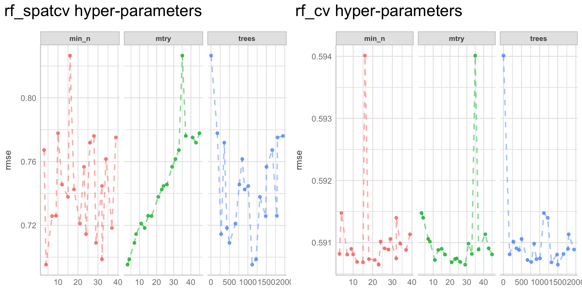
Figure 28: Random forest model (hyper)-parameter tuning combinations - metric: RMSE
XGBoost
Show code
xgboost_hyper_param_plot_spatcv <- readRDS(file = here::here("TidyMod_OUTPUT", "xgboost_hyper_param_plot_spatcv.RDS"))
xgboost_hyper_param_plot_cv <- readRDS(file = here::here("TidyMod_OUTPUT", "xgboost_hyper_param_plot_cv.RDS"))
xgb_hyper_param_plot <-
gridExtra::grid.arrange(xgboost_hyper_param_plot_spatcv + theme(legend.position="none"),
xgboost_hyper_param_plot_cv + theme(legend.position="none"),
ncol = 2)
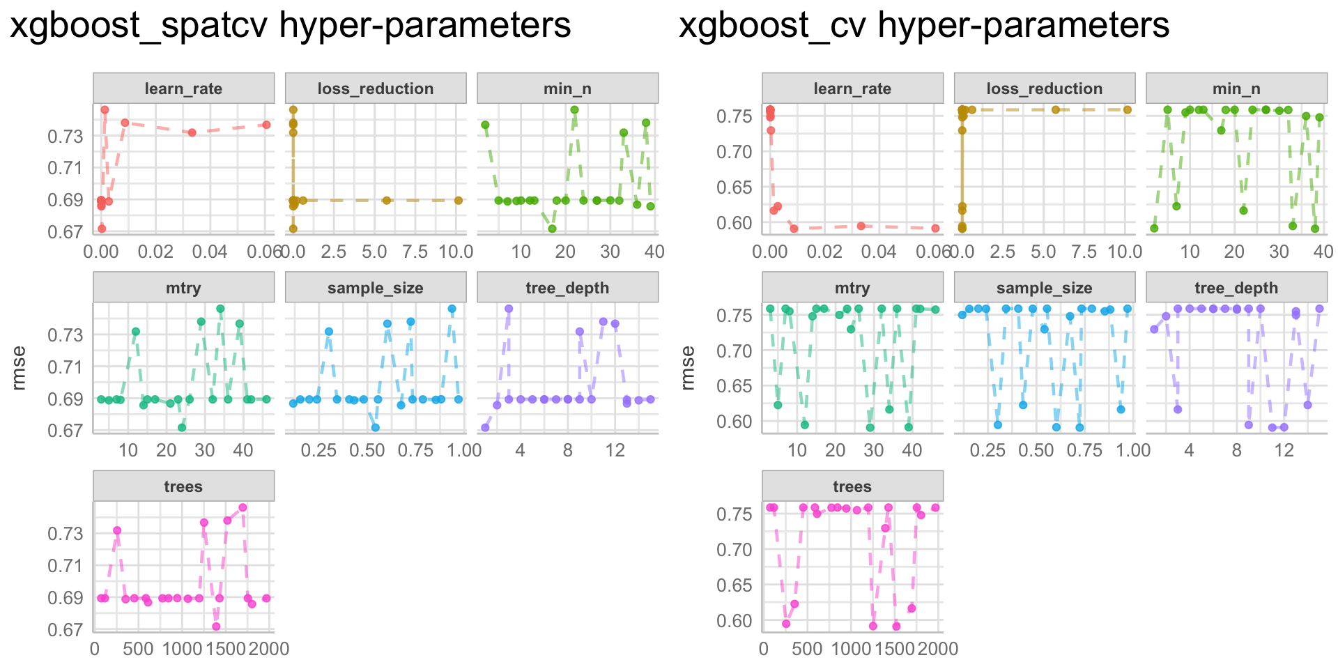
Figure 29: XGBoost model (hyper)-parameter tuning combinations - metric: RMSE
CatBoost
Show code
catboost_hyper_param_plot_spatcv <- readRDS(file = here::here("TidyMod_OUTPUT", "catboost_hyper_param_plot_spatcv.RDS"))
catboost_hyper_param_plot_cv <- readRDS(file = here::here("TidyMod_OUTPUT", "catboost_hyper_param_plot_cv.RDS"))
catboost_hyper_param_plot <-
gridExtra::grid.arrange(catboost_hyper_param_plot_spatcv + theme(legend.position="none"),
catboost_hyper_param_plot_cv + theme(legend.position="none"),
ncol = 2)
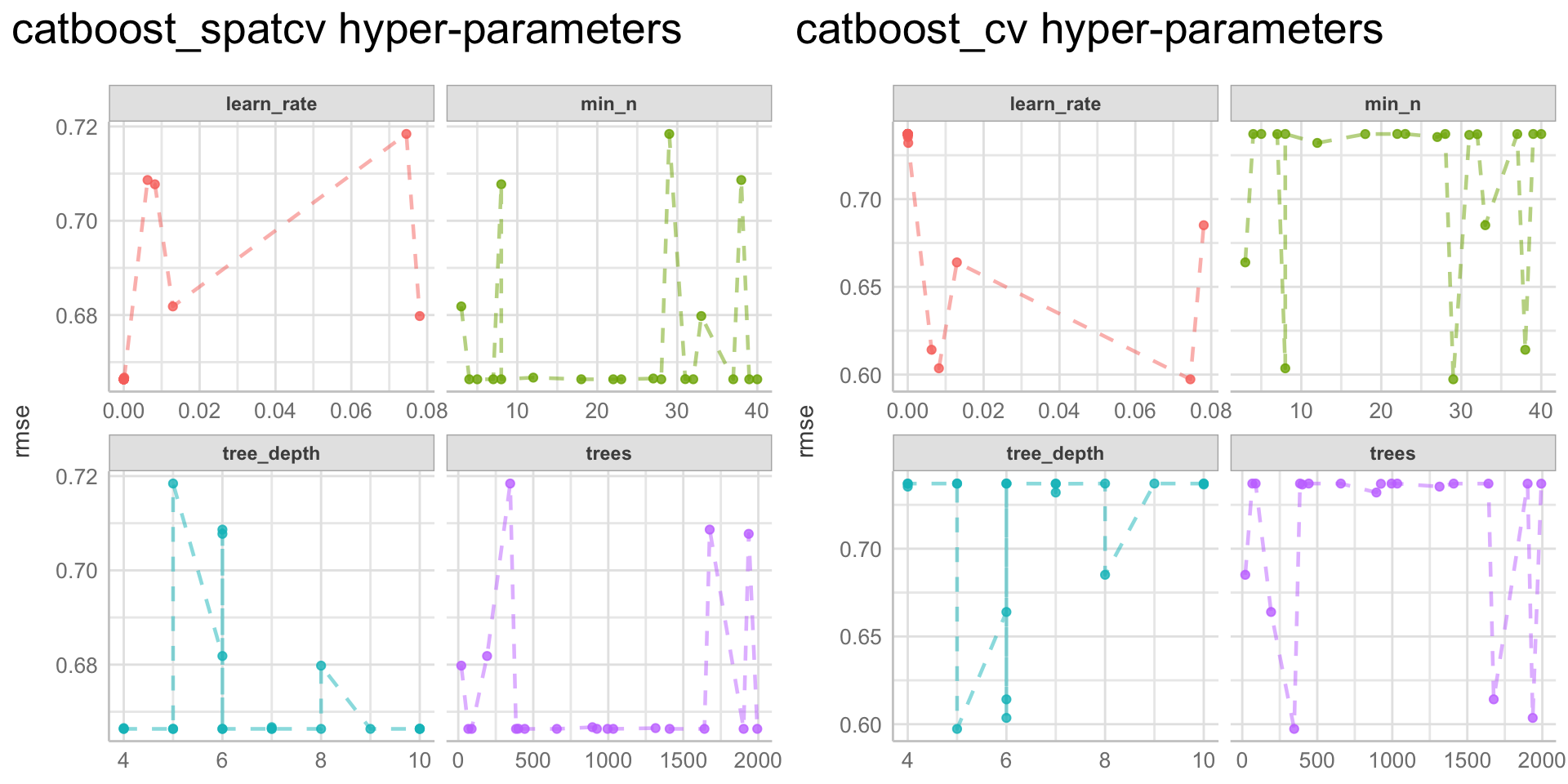
Figure 30: CatBoost model (hyper)-parameter tuning combinations - metric: RMSE
LightGMB
Show code
lightgmb_hyper_param_plot_spatcv <- readRDS(file = here::here("TidyMod_OUTPUT", "lightgmb_param_plot_spatcv.RDS"))
lightgmb_hyper_param_plot_cv <- readRDS(file = here::here("TidyMod_OUTPUT", "lightgmb_param_plot_cv.RDS"))
lightgmb_hyper_param_plot <-
gridExtra::grid.arrange(lightgmb_hyper_param_plot_spatcv + theme(legend.position="none"),
lightgmb_hyper_param_plot_cv + theme(legend.position="none"),
ncol = 2)
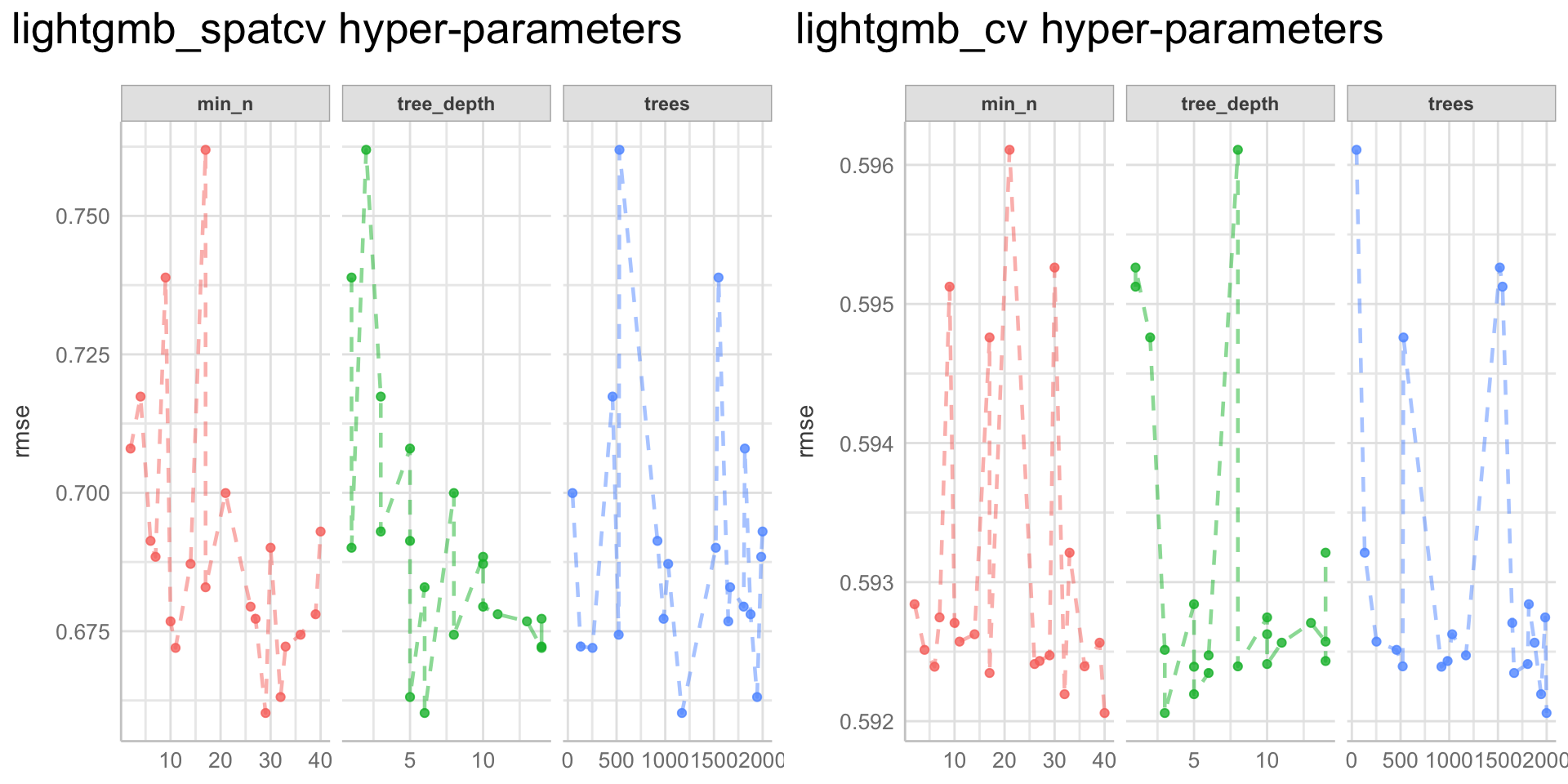
Figure 31: LightGMB model (hyper)-parameter tuning combinations - metric: RMSE
STEP 6: Evaluating model performances
Model results of all models prior to selection of best (hyper)-parameter combinations
################################################################################
# Spatial k-fold cross validation
# ------------------------------------------------------------------------------
# Loading the models from previous model run
lm_fit_spatcv <- readRDS(file = here::here("TidyMod_OUTPUT", "lm_fit_spatcv.RDS"))
glm_fit_spatcv <- readRDS(file = here::here("TidyMod_OUTPUT", "glm_fit_spatcv.rds"))
spline_fit_spatcv <- readRDS(file = here::here("TidyMod_OUTPUT", "spline_fit_spatcv.rds"))
knn_fit_spatcv <- readRDS(file = here::here("TidyMod_OUTPUT", "knn_fit_spatcv.rds"))
pca_fit_spatcv <- readRDS(file = here::here("TidyMod_OUTPUT", "pca_fit_spatcv.rds"))
svm_fit_spatcv <- readRDS(file = here::here("TidyMod_OUTPUT", "svm_fit_spatcv.rds"))
rf_param_fit_spatcv <- readRDS(file = here::here("TidyMod_OUTPUT", "rf_param_fit_spatcv.rds"))
xgboost_param_fit_spatcv <- readRDS(file = here::here("TidyMod_OUTPUT", "xgboost_param_fit_spatcv.rds"))
catboost_param_fit_spatcv <- readRDS(file = here::here("TidyMod_OUTPUT", "catboost_param_fit_spatcv.rds"))
lightgmb_param_fit_spatcv <- readRDS(file = here::here("TidyMod_OUTPUT", "lightgmb_param_fit_spatcv.rds"))
# Create a tibble with all model results ---------------------------------------
model_results_spatcv <- tibble(model = list(lm_fit_spatcv,
glm_fit_spatcv,
spline_fit_spatcv,
knn_fit_spatcv,
pca_fit_spatcv,
svm_fit_spatcv,
rf_param_fit_spatcv,
xgboost_param_fit_spatcv,
catboost_param_fit_spatcv,
lightgmb_param_fit_spatcv),
model_name = c("lm", "glm", "spline", "knn", "pca", "svm", "RF", "XGB", "CatB", "liGMB"))
# Create a helper function for collecting model metrics ------------------------
map_collect_metrics <- function(model){
model %>%
select(id, .metrics) %>%
unnest()
}
# Applying the helper function and extracting the model metrics ----------------
model_results_spatcv <- model_results_spatcv %>%
mutate(res = map(model, map_collect_metrics)) %>%
select(model_name, res) %>%
unnest(res)
# SAVING --------------------------------------------------------------------------------
# Spatial k-fold cross validation
saveRDS(model_results_spatcv, here::here("TidyMod_OUTPUT","model_results_spatcv.RDS"))
################################################################################
# Normal (random) k-fold cross validation (CV-fold)
# ------------------------------------------------------------------------------
# Loading the models from previous model run
lm_fit_cv <- readRDS(file = here::here("TidyMod_OUTPUT", "lm_fit_cv.rds"))
glm_fit_cv <- readRDS(file = here::here("TidyMod_OUTPUT", "glm_fit_cv.rds"))
spline_fit_cv <- readRDS(file = here::here("TidyMod_OUTPUT", "spline_fit_cv.rds"))
knn_fit_cv <- readRDS(file = here::here("TidyMod_OUTPUT", "knn_fit_cv.rds"))
pca_fit_cv <- readRDS(file = here::here("TidyMod_OUTPUT", "pca_fit_cv.rds"))
svm_fit_cv <- readRDS(file = here::here("TidyMod_OUTPUT", "svm_fit_cv.rds"))
rf_param_fit_cv <- readRDS(file = here::here("TidyMod_OUTPUT", "rf_param_fit_cv.rds"))
xgboost_param_fit_cv <- readRDS(file = here::here("TidyMod_OUTPUT", "xgboost_param_fit_cv.rds"))
catboost_param_fit_cv <- readRDS(file = here::here("TidyMod_OUTPUT", "catboost_param_fit_cv.rds"))
lightgmb_param_fit_cv <- readRDS(file = here::here("TidyMod_OUTPUT", "lightgmb_param_fit_cv.rds"))
# Create a tibble with all model results ---------------------------------------
model_results_cv <- tibble(model = list(lm_fit_cv,
glm_fit_cv,
spline_fit_cv,
knn_fit_cv,
pca_fit_cv,
svm_fit_cv,
rf_param_fit_cv,
xgboost_param_fit_cv,
catboost_param_fit_cv,
lightgmb_param_fit_cv),
model_name = c("lm", "glm", "spline", "knn", "pca", "svm", "RF", "XGB", "CatB", "liGMB"))
# Create a helper function for collecting model metrics ------------------------
map_collect_metrics <- function(model){
model %>%
select(id, .metrics) %>%
unnest()
}
# Applying the helper function and extracting the model metrics ----------------
model_results_cv <- model_results_cv %>%
mutate(res = map(model, map_collect_metrics)) %>%
select(model_name, res) %>%
unnest(res)
# SAVING --------------------------------------------------------------------------------
# Normal (random) k-fold cross validation (CV-fold)
saveRDS(model_results_cv, here::here("TidyMod_OUTPUT","model_results_cv.RDS"))
Visualising model performances with boxplots
Defining a custom colours range
Show code
nb.cols.10 <- 10
af.ml.colors.10 <- colorRampPalette(brewer.pal(8, "Set2"))(nb.cols.10)
nb.cols.9 <- 9
af.ml.colors.9 <- colorRampPalette(brewer.pal(8, "Set2"))(nb.cols.9)
Models tuned/fit with spatial clustiering cv-folds
Show code
################################################################################
# Spatial k-fold cross validation
# ------------------------------------------------------------------------------
# Loading the models
model_results_spatcv <- readRDS(file = here::here("TidyMod_OUTPUT","model_results_spatcv.RDS"))
model_results_all_plot_spatcv <- model_results_spatcv %>%
dplyr::filter(.estimate < 2) %>% # <- Its necessary to filter the metric estimates!
ggplot(aes(x = model_name, y = .estimate, color = model_name)) +
geom_boxplot(fill = "white", alpha = 0.8, size = 2) +
geom_jitter(width = 0.2, height = 0.2) +
scale_color_manual(values = af.ml.colors.10) +
facet_wrap(~.metric, scales = "free_y") +
see::theme_lucid(axis.text.angle = 45, plot.title.size = 20) +
ggtitle("Evaluation of models tuned/fit with spatial clustering cv-folds - all metrics")
# Plotting
model_results_all_plot_spatcv
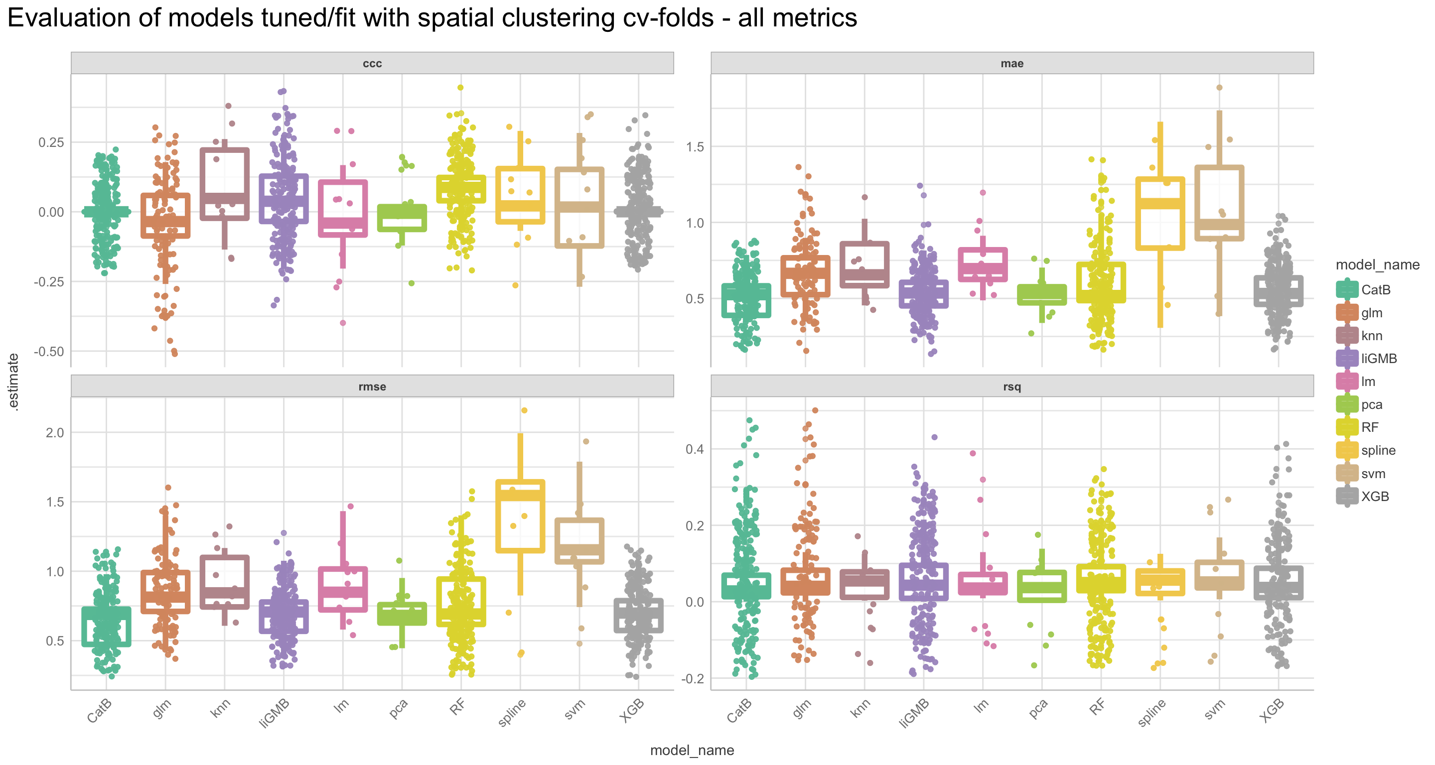
Figure 32: Model evaluation, resampling: Spatial clustering cv-folds - metrics: CCC, RMSE, MAE, rsq
Models tuned/fit with normal cv-folds
Show code
################################################################################
# Normal (random) k-fold cross validation (CV-fold)
# ------------------------------------------------------------------------------
# Loading the models
model_results_cv <- readRDS(file = here::here("TidyMod_OUTPUT","model_results_cv.RDS"))
model_results_all_plot_cv <- model_results_cv %>%
dplyr::filter(.estimate < 2) %>% # <- Its necessary to filter the metric estimates!
ggplot(aes(x = model_name, y = .estimate, color = model_name)) +
geom_boxplot(fill = "white", alpha = 0.8, size = 2) +
geom_jitter(width = 0.2, height = 0.2) +
scale_color_manual(values = af.ml.colors.10) +
facet_wrap(~.metric, scales = "free_y") +
see::theme_lucid(axis.text.angle = 45, plot.title.size = 20) +
ggtitle("Evaluation of models tuned/fit with normal cv-folds - all metrics")
# ------------------------------------------------------------------------------
# Plotting
model_results_all_plot_cv
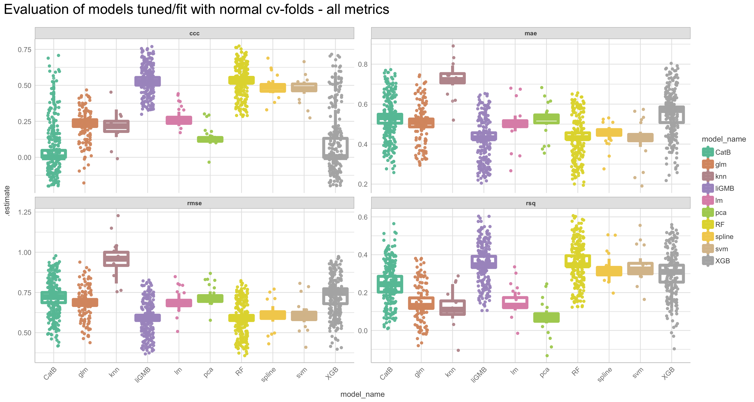
Figure 33: Model evaluation, resampling: Normal cv-folds - metrics: CCC, RMSE, MAE, rsq
We see that the simpler models, e.g. lm and spline perform relatively good compared to the more complex (tree-based models). However, because we did not select best performing (hyper)-parameters yet we see that the tree-based models have instances that do perform much better.
Variability in folds for the different models
Show code
################################################################################
# Spatial k-fold cross validation
model_evaluation_fold_variability_plot_spatcv <-
model_results_spatcv %>%
dplyr::filter(.estimate < 5) %>%
ggplot(aes(x = model_name, y = .estimate, color = id, group = id)) +
geom_line(size = 1.5, alpha = 0.8) +
facet_wrap(~.metric, scales = "free_y") +
scale_color_manual(values = af.ml.colors.10) +
see::theme_lucid(axis.text.angle = 45, plot.title.size = 20) +
ggtitle("Variability in metrics between each cv-fold for all tested models, resampling: Spatial clustering cv-folds")
model_evaluation_fold_variability_plot_spatcv
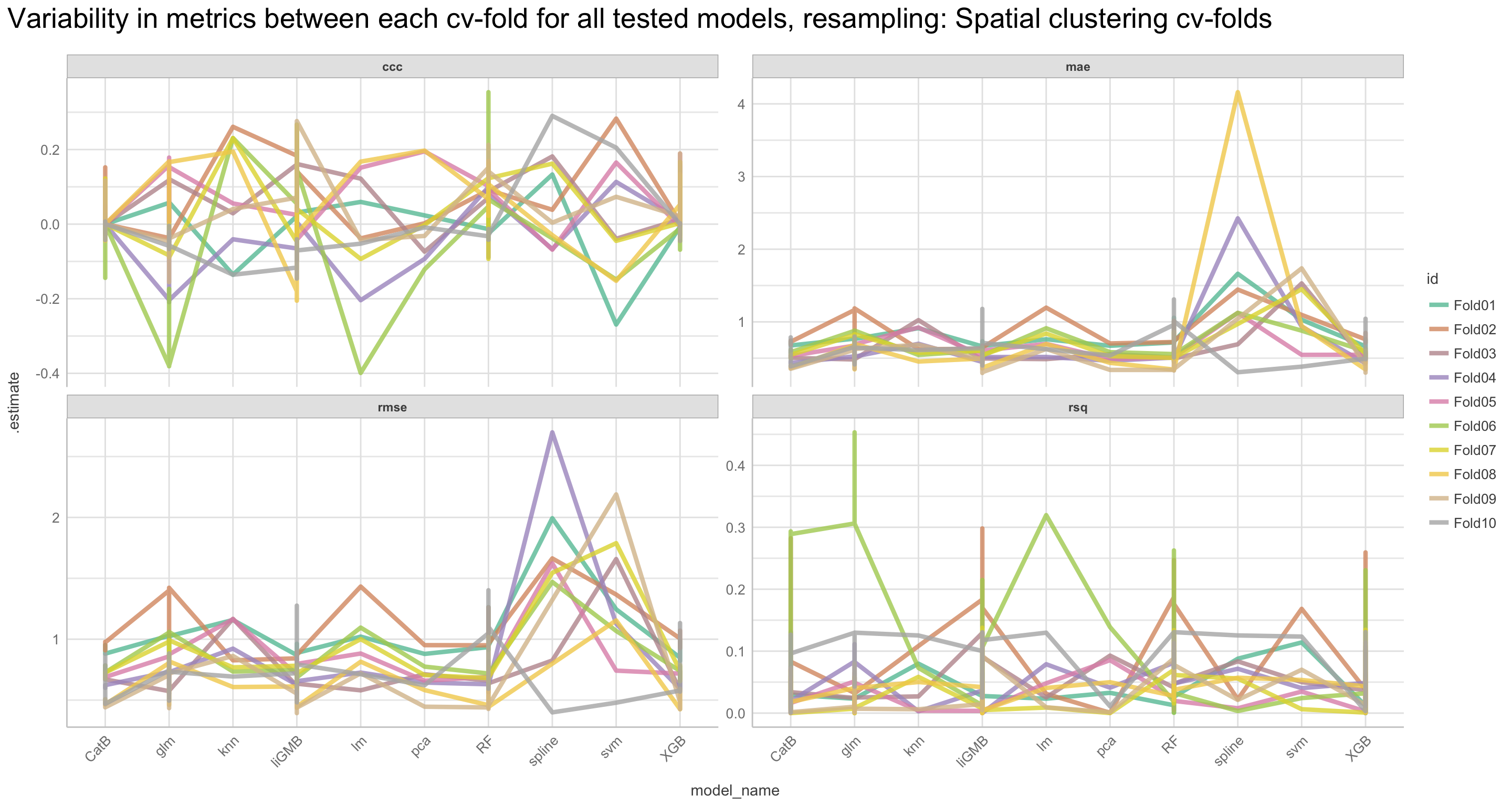
Figure 34: Variability in metrics between each cv-fold for all tested models, resampling: Spatial clustering cv-folds - metrics: CCC, RMSE, MAE, rsq
Show code
################################################################################
# Normal (random) k-fold cross validation (CV-fold)
model_evaluation_fold_variability_plot_cv <-
model_results_cv %>%
dplyr::filter(.estimate < 5) %>%
ggplot(aes(x = model_name, y = .estimate, color = id, group = id)) +
geom_line(size = 1.5, alpha = 0.8) +
facet_wrap(~.metric, scales = "free_y") +
scale_color_manual(values = af.ml.colors.10) +
see::theme_lucid(axis.text.angle = 45, plot.title.size = 20) +
ggtitle("Variability in metrics between each cv-fold for all tested models, resampling: Normal cv-folds")
model_evaluation_fold_variability_plot_cv
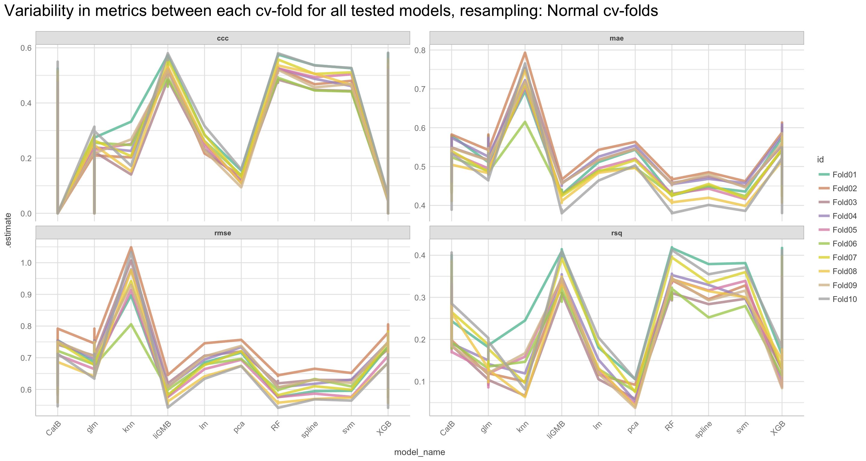
Figure 35: Variability in metrics between each cv-fold for all tested models, resampling: Normal cv-folds - metrics: CCC, RMSE, MAE, rsq
We see a large variability in some of the models, especially the spline model - hence it might perform well in general, but there are large differences between the folds, that we have to be aware of.
Variability in metric suitability for the different model comparisons
Show code
################################################################################
# Spatial k-fold cross validation
model_metric_suitability_density_plot_spatcv <-
model_results_spatcv %>%
dplyr::filter(.estimate < 5) %>%
ggplot(aes(x = .estimate, color = model_name, fill = model_name)) +
geom_density(alpha = 0.1, size = 1) +
facet_wrap(~.metric, scales = "free") +
scale_color_manual(values = af.ml.colors.10) +
scale_fill_manual(values = af.ml.colors.10) +
see::theme_lucid(plot.title.size = 20) +
ggtitle("Metric suitability density plot for all tested models, resampling: Spatial clustering cv-folds") +
xlab("Estimated logRR values") +
ylab("Density")
model_metric_suitability_density_plot_spatcv
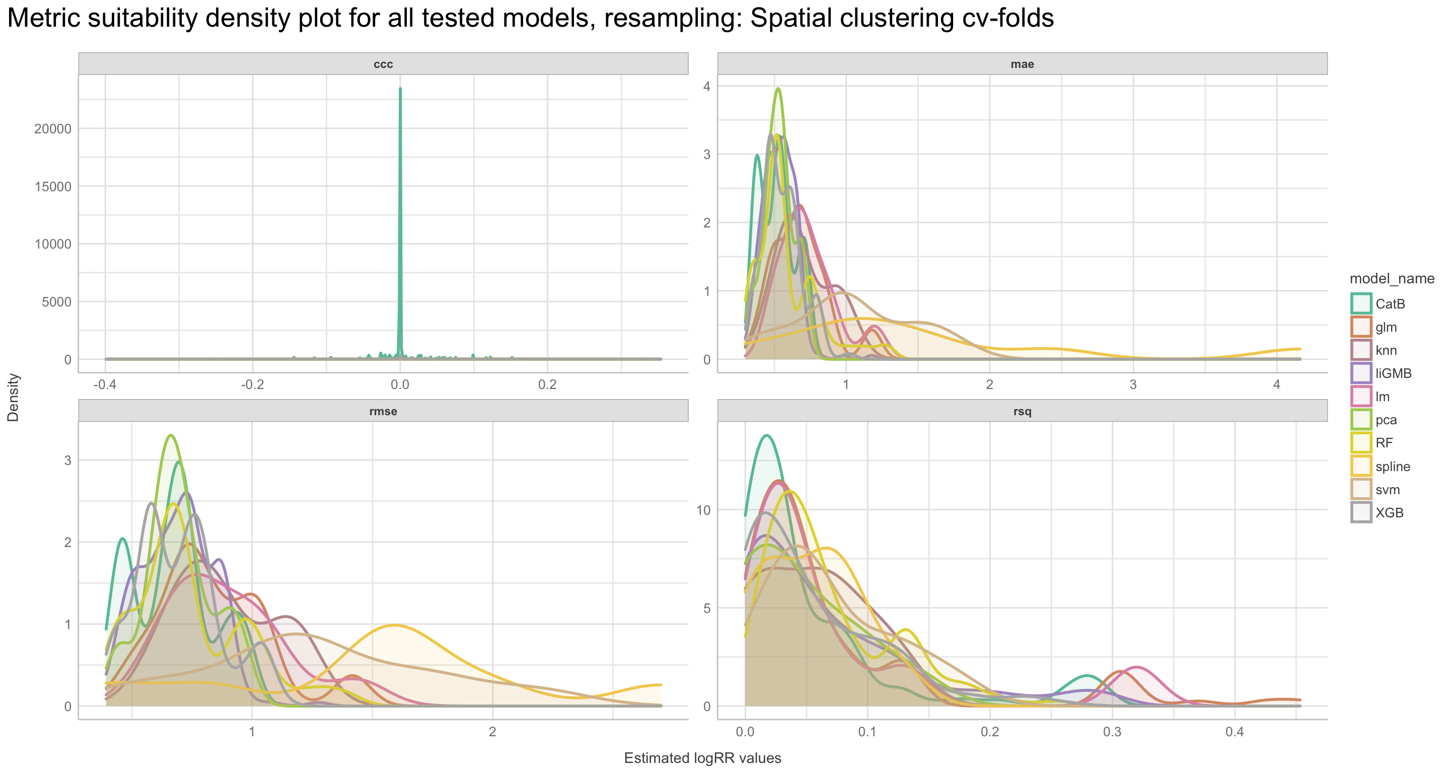
Figure 36: Density plot of metric suitability for all tested models, resampling: Spatial clustering cv-folds - metrics: CCC, RMSE, MAE, rsq
It seems like the spline and kNN models is outperforming many of the other models based on the RMSE metric - as these models have the lowest value for RMSE. However, their spread is not very good. They seem to both be generally over-estimating logRR values, compared to the other models. This is why it is extremely powerful to have more than one metric when comparing these machine learning modelling algorithms. Because one model might outperform other models in one aspect but not on other, more generally important aspects. Keep this in mind!
Show code
################################################################################
# Normal (random) k-fold cross validation (CV-fold)
model_metric_suitability_density_plot_cv <-
model_results_cv %>%
dplyr::filter(.estimate < 5) %>%
ggplot(aes(x = .estimate, color = model_name, fill = model_name)) +
geom_density(alpha = 0.1, size = 1) +
facet_wrap(~.metric, scales = "free") +
scale_color_manual(values = af.ml.colors.10) +
scale_fill_manual(values = af.ml.colors.10) +
see::theme_lucid(plot.title.size = 20) +
ggtitle("Metric suitability density plot for all tested models, resampling: Normal cv-folds") +
xlab("Estimated logRR values") +
ylab("Density")
model_metric_suitability_density_plot_cv
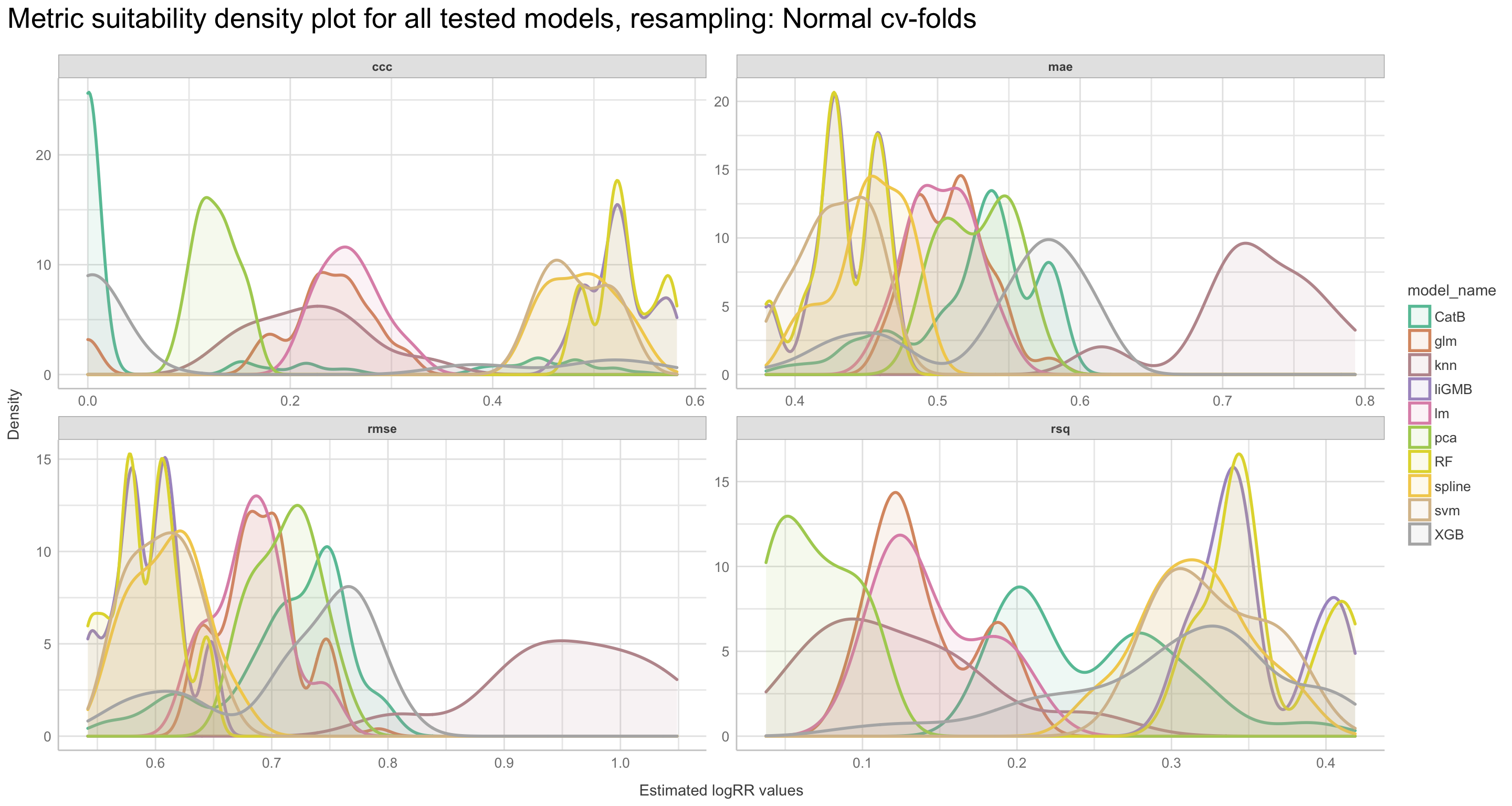
Figure 37: Density plot of metric suitability for all tested models, resampling: Normal cv-folds - metrics: CCC, RMSE, MAE, rsq
There are large differences in the estimate density distributions for the different models. Yet, the RMSE seems to be a reasonable metric. However, there seem to be no metric that really suits our data. We can decide to continue to make use of RMSE and MAE as these are generally used for regression problems.
Note: Pay attention to how different the desity distribution is for all metrics when comparing the two different resampling techniques, spatial clustering cv-folds and the normal cv-folds.
If we recall again the logRR distribution, that is a little positively skewed, it is easier to interpret the metric suitability density plots. Optimally we are interested in metrics that cover the whole “real” distribution of logRR.
Show code
logRR_distribution <- agrofor.biophys.modelling.data %>%
rationalize(logRR) %>%
drop_na(logRR) %>%
ggplot(aes(x = logRR)) +
geom_density(aes(y = ..count..), fill = "lightgray") +
geom_vline(aes(xintercept = mean(logRR)),
linetype = "dashed",
size = 1, color = "#FC4E07") +
scale_x_continuous(name="Observed logRR values", limits=c(-2.5, 2.5)) +
ggtitle("Density/count distribution of real logRR values for the ERA agroforestry data") +
ylab("Count (number of oblersavions)") +
see::theme_lucid()
logRR_distribution
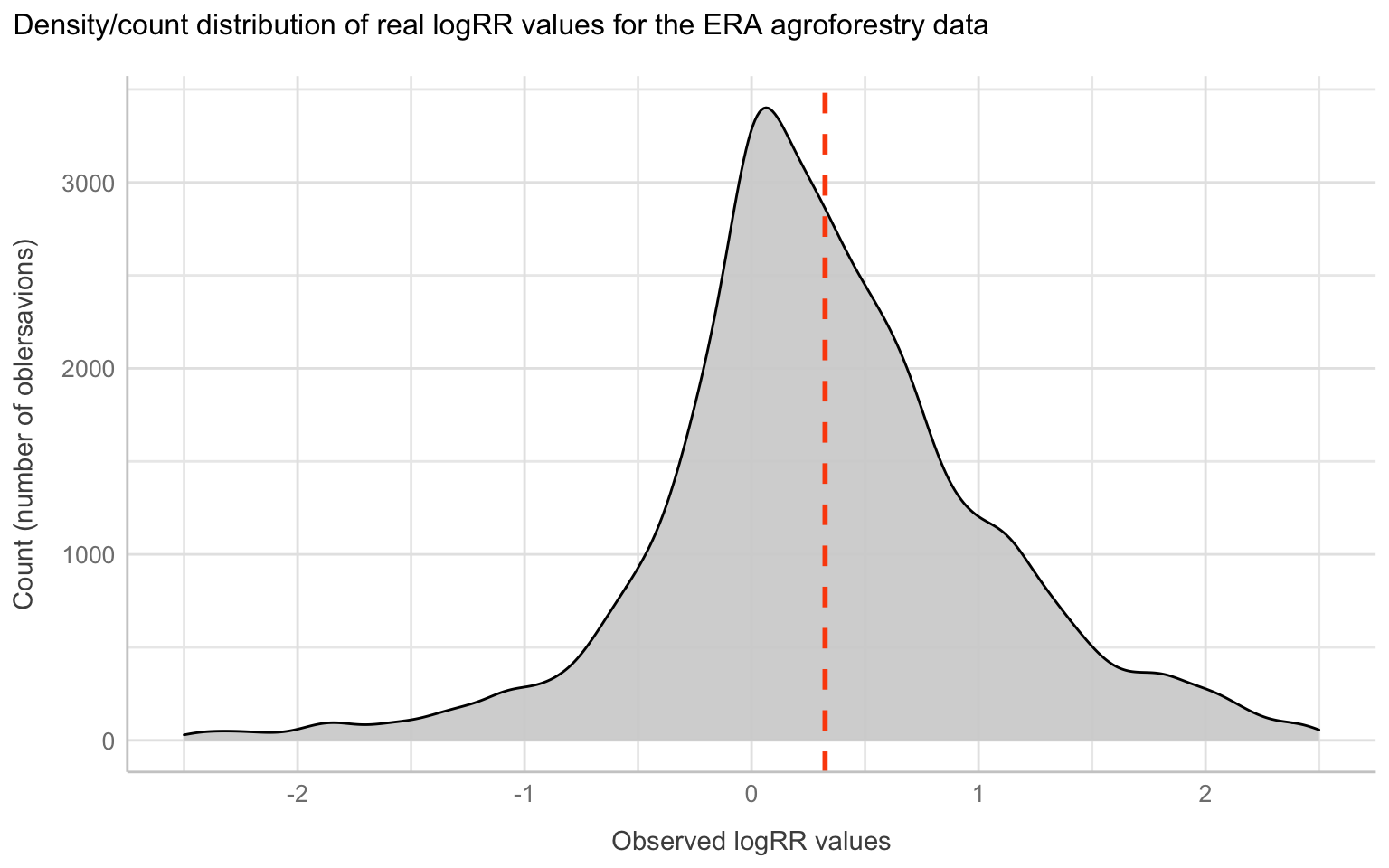
Figure 38: Density/count distribution of real logRR values
Show code
#Warning: Removed 78 rows containing non-finite values (stat_density).
Summerising model metric performances
Show code
################################################################################
# Spatial k-fold cross validation
model_results_spatcv %>%
dplyr::filter(.metric == "rmse") %>%
mutate_if(sapply(model_results_spatcv, is.character), as.factor) %>%
group_by(model_name, .metric) %>%
summarise(mean = mean(.estimate)) %>%
arrange(desc(-mean)) %>%
ggplot() +
geom_bar(aes(x = reorder(model_name, mean), y = mean), stat = 'identity') +
ggtitle("Mean RMSE metric for all tested models, resampling: Normal cv-folds") +
ylab("Mean RMSE") +
xlab("Model") +
see::theme_lucid()
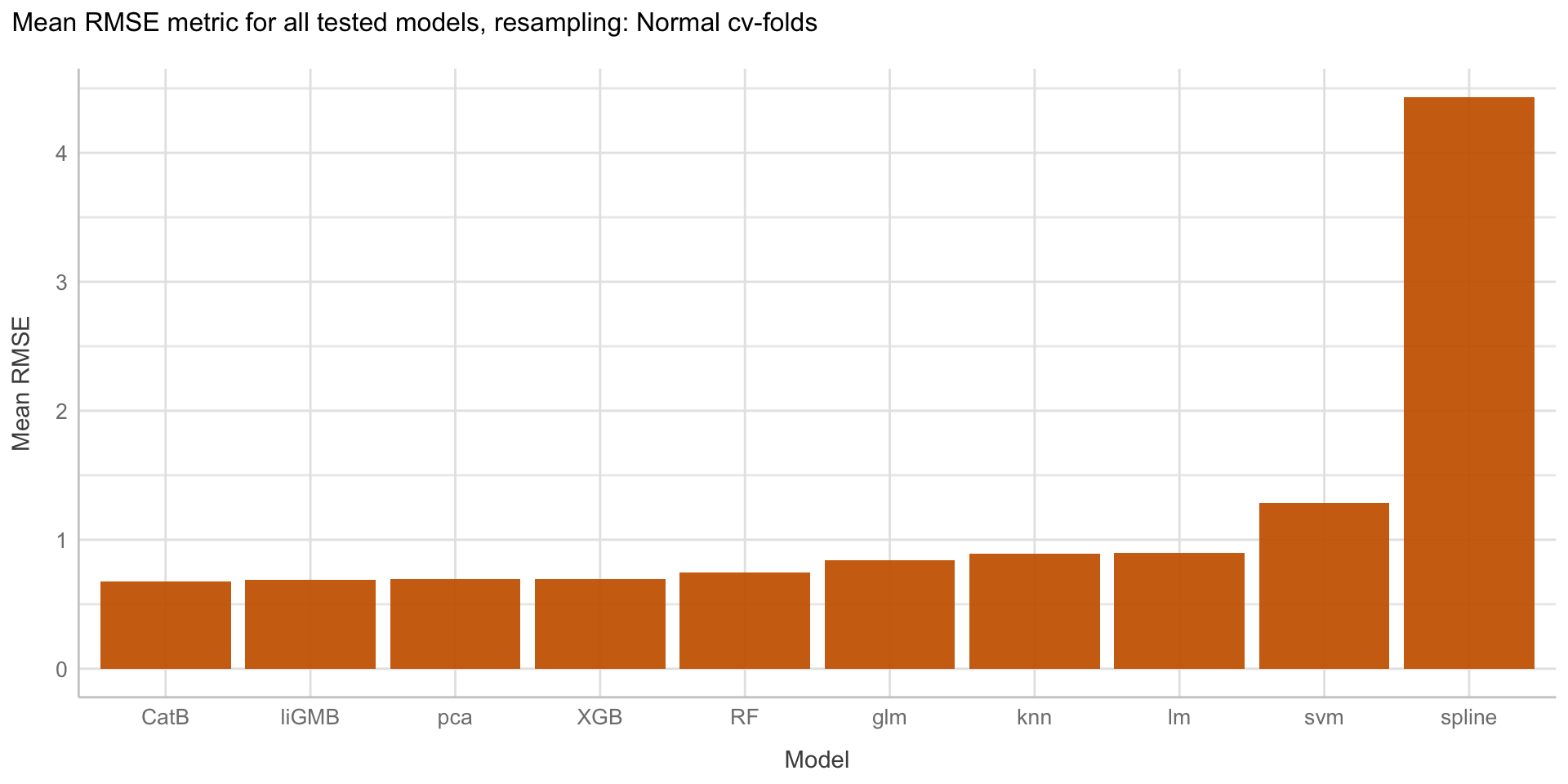
Figure 39: Summarising model metric performances, resampling: Spatial clustering cv-folds - metric: RMSE
Show code
################################################################################
# Normal (random) k-fold cross validation (CV-fold)
model_results_cv %>%
dplyr::filter(.metric == "rmse") %>%
mutate_if(sapply(model_results_cv, is.character), as.factor) %>%
group_by(model_name, .metric) %>%
summarise(mean = mean(.estimate)) %>%
arrange(desc(-mean)) %>%
ggplot() +
geom_bar(aes(x = reorder(model_name, mean), y = mean), stat = 'identity') +
ggtitle("Mean RMSE metric for all tested models, resampling: Normal cv-folds") +
ylab("Mean RMSE") +
xlab("Model") +
see::theme_lucid()
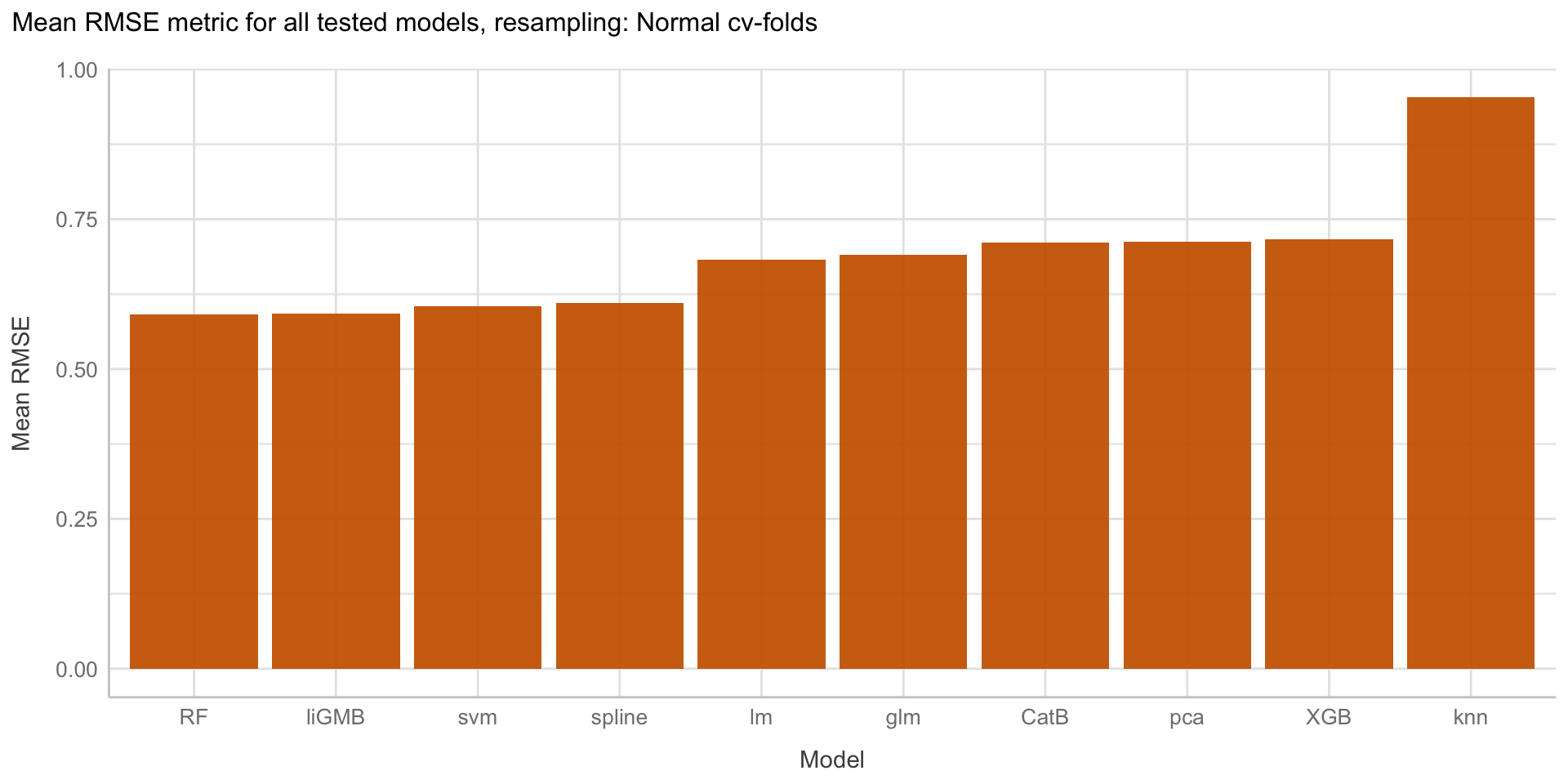
Figure 40: Summarising model metric performances, resampling: Normal cv-folds - metric: RMSE
Even though the spline model(s) does seem to be superior on all the metrics, we know that its “accuracy” is relatively weak, as we saw the variations between the folds and its density distributions. Hence, the subsequent best models based on best performing (hyper)-parameter combinations are probably more appropriate to use.
Using tidyposterior for model comparisons
We can use the package tidyposterior, part of the tidymodels meta-package, to get a better insight into how the individual models perform post-hoc using Bayesian generalised linear models. cThis is useful when one wants to conduct a post-hoc analyses of resampling results generated by the various models. For example, if two models are evaluated using the root mean squared error (RMSE) metric on our 10-fold cross-validation, there are 10 paired statistics (one for each fold). These can be used to make comparisons between models without involving a test set. Hence, we get a picture on the variation in a specific metric for the models across the different folds.
First, calculating the posterior distributions
The tidyposterior package uses the Stan software for specifying and fitting the models via the rstanarm package.
# library(tidyposterior)
################################################################################
# Spatial k-fold cross validation
model_posterior_spatcv <-
model_results_spatcv %>%
filter(.metric == "rmse") %>%
select(model_name, id, .estimate) %>%
pivot_wider(names_from = "model_name", values_from = ".estimate", values_fn = mean)
rmse_model_spatcv <- tidyposterior::perf_mod(model_posterior_spatcv, seed = 412)
# ----------SAVING ----------------- ----------------- ----------------- -----------------
saveRDS(rmse_model_spatcv, file = here::here("TidyMod_OUTPUT", "rmse_model_spatcv.RDS"))
# library(tidyposterior)
################################################################################
# Normal (random) k-fold cross validation (CV-fold)
model_posterior_cv <-
model_results_cv %>%
filter(.metric == "rmse") %>%
select(model_name, id, .estimate) %>%
pivot_wider(names_from = "model_name", values_from = ".estimate", values_fn = mean)
rmse_model_cv <- tidyposterior::perf_mod(model_posterior_cv, seed = 421)
# ----------SAVING ----------------- ----------------- ----------------- -----------------
saveRDS(rmse_model_cv, file = here::here("TidyMod_OUTPUT", "rmse_model_cv.RDS"))
################################################################################
# Spatial k-fold cross validation
# Reading data
rmse_model_spatcv <- readRDS(file = here::here("TidyMod_OUTPUT", "rmse_model_spatcv.RDS"))
rmse_model_spatcv %>% tidy() %>% group_by(model) %>% summarise(mean = mean(posterior))
# A tibble: 10 × 2
model mean
<chr> <dbl>
1 CatB 0.684
2 glm 0.865
3 knn 0.899
4 liGMB 0.685
5 lm 0.907
6 pca 0.722
7 RF 0.736
8 spline 4.44
9 svm 1.31
10 XGB 0.706################################################################################
# Normal (random) k-fold cross validation (CV-fold)
# Reading data
rmse_model_cv <- readRDS(file = here::here("TidyMod_OUTPUT", "rmse_model_cv.RDS"))
rmse_model_cv %>% tidy() %>% group_by(model) %>% summarise(mean = mean(posterior))
# A tibble: 10 × 2
model mean
<chr> <dbl>
1 CatB 0.710
2 glm 0.690
3 knn 0.953
4 liGMB 0.593
5 lm 0.682
6 pca 0.712
7 RF 0.590
8 spline 0.610
9 svm 0.605
10 XGB 0.716The posterior distribution is useful to determine if there is in fact a difference between the models (for the metric used, e.g. RMSE). The posterior distribution shows the distribution of the difference in metrics between the models. Whether it is higher or lower depends on the metric one choose to use (RMSE, ROC_AUC, etc.). If the distribution’s central tendency is not 0 then there is a difference between the models.
Visualising the posterior distribution with ggplot
We can now visualize the posterior distribution of the models by plotting it with ggplot
Show code
################################################################################
# Spatial k-fold cross validation
post_plot_rmse_model_spatcv <-
rmse_model_spatcv %>% tidy() %>%
ggplot(aes(x = model, y = posterior, color = model)) +
geom_violin() +
geom_quasirandom(dodge.width = 0.3, varwidth = FALSE, width = 0.08, alpha = 0.05) +
stat_summary(fun.y = "median", geom = "point", size = 2, color = "black") +
stat_summary(fun.y = "median", geom = "line", aes(group = 1), size = 1.1, color = "black") +
scale_color_manual(values = af.ml.colors.10) +
ggtitle("Posterior distributions for all tested models, resampling: Spatial clustering cv-folds - metric: RMSE") +
ylab("Mean RMSE") +
xlab("Model") +
see::theme_lucid(axis.text.angle = 45, plot.title.size = 20, legend.title.size = 15, legend.text.size = 15, axis.text.size = 15, tags.size = 15, legend.position = "bottom")
post_plot_rmse_model_spatcv
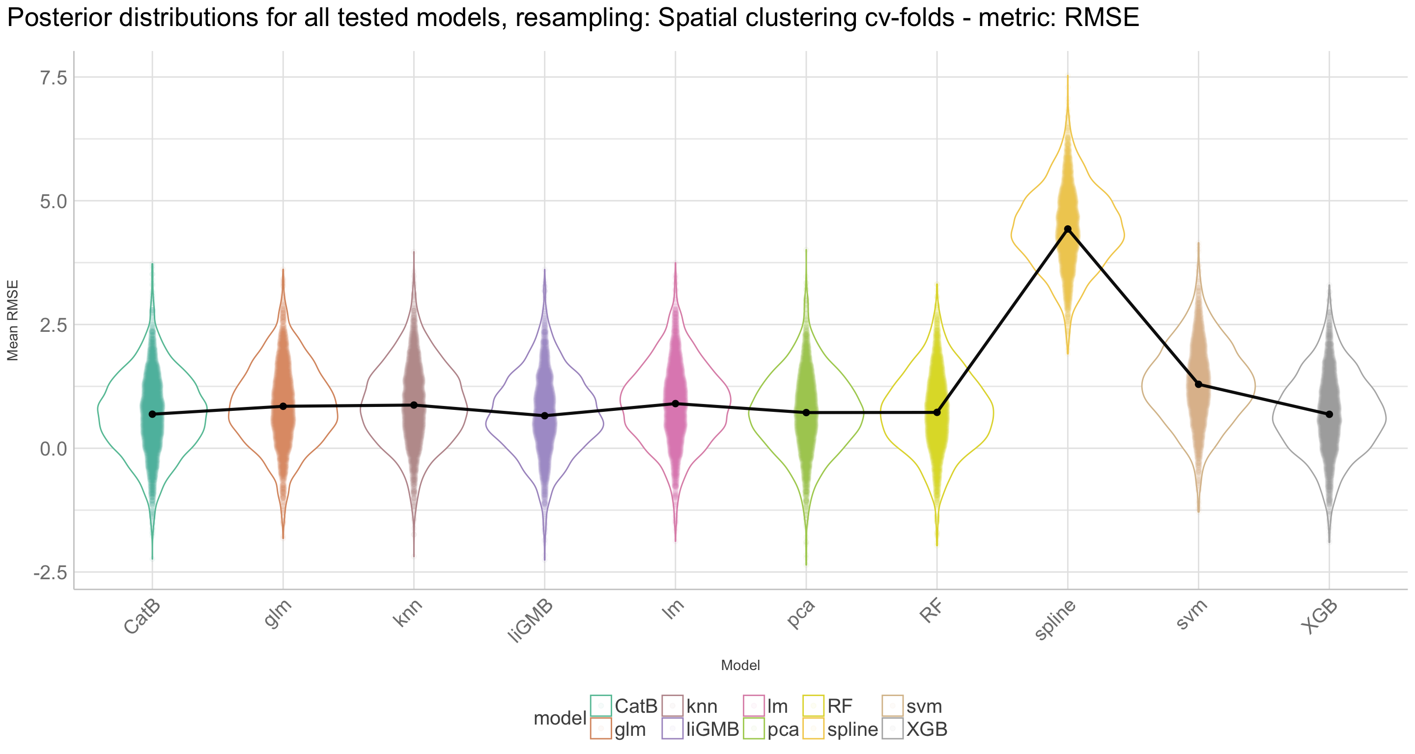
Figure 41: Posterior distributions for all tested models, resampling: Spatial clustering cv-folds - metric: RMSE
Show code
################################################################################
# Normal (random) k-fold cross validation (CV-fold)
post_plot_rmse_model_cv <-
rmse_model_cv %>% tidy() %>%
ggplot(aes(x = model, y = posterior, color = model)) +
geom_violin() +
geom_quasirandom(dodge.width = 0.3, varwidth = FALSE, width = 0.08, alpha = 0.05) +
stat_summary(fun.y = "median", geom = "point", size = 2, color = "black") +
stat_summary(fun.y = "median", geom = "line", aes(group = 1), size = 1.1, color = "black") +
scale_color_manual(values = af.ml.colors.10) +
ggtitle("Posterior distributions for all tested models, resampling: Spatial clustering cv-folds - metric: RMSE") +
ylab("Mean RMSE") +
xlab("Model") +
see::theme_lucid(axis.text.angle = 45, plot.title.size = 20, legend.title.size = 15, legend.text.size = 15, axis.text.size = 15, tags.size = 15, legend.position = "bottom")
post_plot_rmse_model_cv
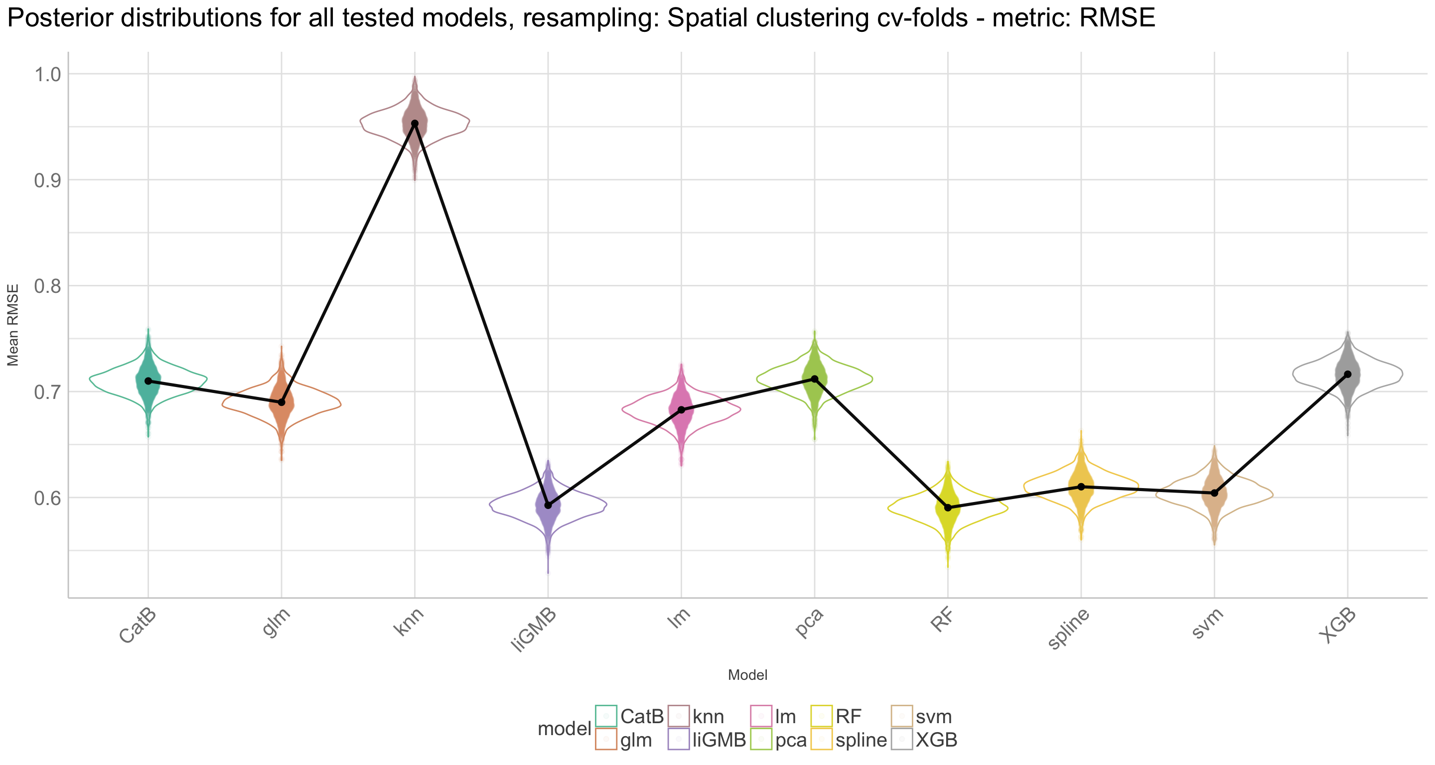
Figure 42: Posterior distributions for all tested models, resampling: Normal cv-folds - metric: RMSE
These posterior distribution plots are very interesting because they give us a detailed insight into how the models differ from each other. We also see that there are significant differences between the models whether we use spatial clustering cv-folds or normal cv-folds.
Contrast assessment between the models
Finalluy, we can use the contrast assessment between models to understand the
################################################################################
# Spatial k-fold cross validation
contrast_models(rmse_model_spatcv)
# Posterior samples of performance differences
# A tibble: 180,000 × 4
difference model_1 model_2 contrast
<dbl> <chr> <chr> <chr>
1 -0.728 lm glm lm vs. glm
2 -0.308 lm glm lm vs. glm
3 0.385 lm glm lm vs. glm
4 1.43 lm glm lm vs. glm
5 0.734 lm glm lm vs. glm
6 -0.378 lm glm lm vs. glm
7 0.469 lm glm lm vs. glm
8 -0.479 lm glm lm vs. glm
9 -0.738 lm glm lm vs. glm
10 1.13 lm glm lm vs. glm
# … with 179,990 more rows################################################################################
# Normal (random) k-fold cross validation (CV-fold)
contrast_models(rmse_model_cv) %>%
group_by(contrast) %>%
summarise(mean = mean(difference)) %>%
arrange(desc(mean))
# A tibble: 45 × 2
contrast mean
<chr> <dbl>
1 knn vs. RF 0.363
2 knn vs. liGMB 0.360
3 knn vs. svm 0.348
4 knn vs. CatB 0.243
5 knn vs. pca 0.241
6 knn vs. XGB 0.237
7 XGB vs. liGMB 0.124
8 pca vs. RF 0.121
9 pca vs. liGMB 0.119
10 CatB vs. liGMB 0.117
# … with 35 more rowsVisually showcase of the model contrast assessment
These plots might be a little difficult to interpret but basically they show how different each model is compared to another and also how much better or worse this model is. The x-axis shows the difference for the model and this is centered around xero. If the difference is skewed towards the right then the difference is positive ant it can be said that the given model performs better than the one it’s compared with. The y-axis shows the actual posterior probability. Let’s take the example of the glm model. First look at the top row, this will tell you how much better/worse the glm model is compared to the CatBoost model. In this case the glm model does not really have a strong right skewed distribution difference, indicating that it is not ‘significantly’ different from the CatBoost model. However, it is slightly skewed towards the right, suggesting that it is better. The models that have a positive (above zero) location have a significant better performance!
With spatial clustering cv-folds
Show code
################################################################################
# Spatial k-fold cross validation
contrast_plot_rmse_spatcv <- contrast_models(rmse_model_spatcv)
autoplot(contrast_plot_rmse_spatcv)
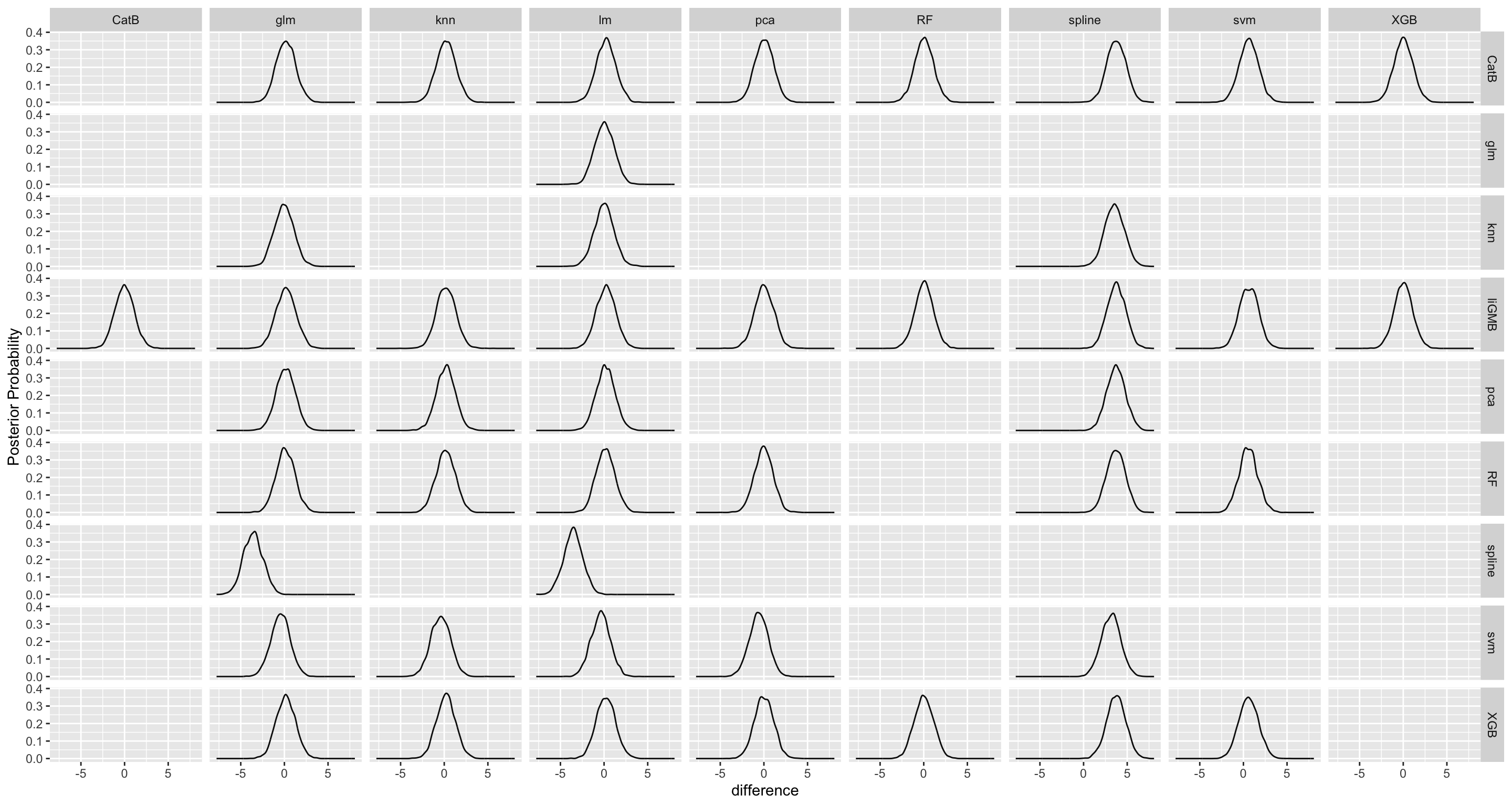
Figure 43: Posterior model contrast assessment, resampling: Spatial clustering cv-folds - metric: RMSE
With normal cv-folds
This picture changes remarkebly when using normal cv-folds as we see below:
Show code
################################################################################
# Normal (random) k-fold cross validation (CV-fold)
contrast_plot_rmse_cv <- contrast_models(rmse_model_cv)
autoplot(contrast_plot_rmse_cv)
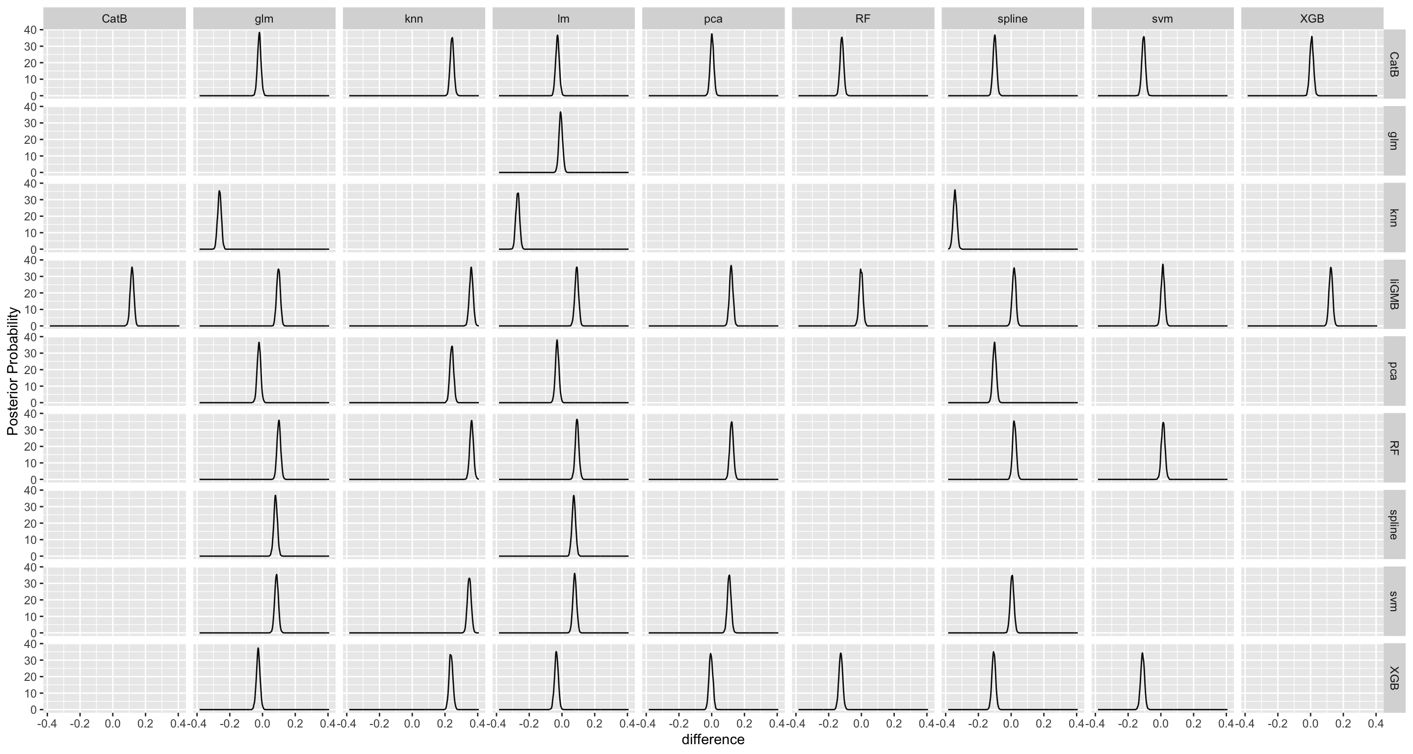
Figure 44: Posterior model contrast assessment, resampling: Normal cv-folds - metric: RMSE
STEP 8: Finalizing models and model workflows
Now we have gained significantly detailed information on all the tested models. Until now, we have only been looking at all (hyper)-parameter fitting/tuning combinations, and we have seen than even within a single model there is enormous differences in the model performance, even across and within our selected metrics. Hence we have not yet selected the best performing (hyper)-paramenter combinations, that result in best performing models. It is now time to do exactly that!
Note: We can update (or “finalize”) our model or workflow objects with settings or values from select_best().
Let us first finalize models and workflows from the non-tree based models as this is a little easier.
Finalizing model workflows for non-tree based models
##########################################################################
# Spatial k-fold cross validation
# Loading models and workflows
#-------------------------------------------------------
lm_fit_spatcv <- readRDS(file = here::here("TidyMod_OUTPUT","lm_fit_spatcv.RDS"))
lm_wf <- readRDS(file = here::here("TidyMod_OUTPUT","lm_wf.RDS"))
glm_fit_spatcv <- readRDS(file = here::here("TidyMod_OUTPUT","glm_fit_spatcv.RDS"))
glm_wf <- readRDS(file = here::here("TidyMod_OUTPUT","glm_wf.RDS"))
spline_fit_spatcv <- readRDS(file = here::here("TidyMod_OUTPUT","spline_fit_spatcv.RDS"))
spline_wf <- readRDS(file = here::here("TidyMod_OUTPUT","spline_wf.RDS"))
knn_fit_spatcv <- readRDS(file = here::here("TidyMod_OUTPUT","knn_fit_spatcv.RDS"))
knn_wf <- readRDS(file = here::here("TidyMod_OUTPUT","knn_wf.RDS"))
pca_fit_spatcv <- readRDS(file = here::here("TidyMod_OUTPUT","pca_fit_spatcv.RDS"))
pca_wf <- readRDS(file = here::here("TidyMod_OUTPUT","pca_wf.RDS"))
svm_fit_spatcv <- readRDS(file = here::here("TidyMod_OUTPUT","svm_fit_spatcv.RDS"))
svm_wf <- readRDS(file = here::here("TidyMod_OUTPUT","svm_wf.RDS"))
# linear (lm) model
#-------------------------------------------------------
# Best and last model
lm_best_rmse_spatcv <- lm_fit_spatcv %>%
tune::select_best("rmse")
# Last model workflow
lm_final_wf_rmse_spatcv <- lm_wf %>%
finalize_workflow(lm_best_rmse_spatcv)
# glm model
#-------------------------------------------------------
# Best and last model
glm_best_rmse_spatcv <- glm_fit_spatcv %>%
tune::select_best("rmse")
# Last model workflow
glm_final_wf_rmse_spatcv <- glm_wf %>%
finalize_workflow(glm_best_rmse_spatcv)
# spline model
#-------------------------------------------------------
# Best and last model
spline_best_rmse_spatcv <- spline_fit_spatcv %>%
tune::select_best("rmse")
# Last model workflow
spline_final_wf_rmse_spatcv <- spline_wf %>%
finalize_workflow(spline_best_rmse_spatcv)
# knn model
#-------------------------------------------------------
# Best and last model
knn_best_rmse_spatcv <- knn_fit_spatcv %>%
tune::select_best("rmse")
# Last model workflow
knn_final_wf_rmse_spatcv <- knn_wf %>%
finalize_workflow(knn_best_rmse_spatcv)
# pca model
#-------------------------------------------------------
# Best and last model
pca_best_rmse_spatcv <- pca_fit_spatcv %>%
tune::select_best("rmse")
# Last model workflow
pca_final_wf_rmse_spatcv <- pca_wf %>%
finalize_workflow(pca_best_rmse_spatcv)
# svm model
#-------------------------------------------------------
# Best and last model
svm_best_rmse_spatcv <- svm_fit_spatcv %>%
tune::select_best("rmse")
# Last model workflow
svm_final_wf_rmse_spatcv <- svm_wf %>%
finalize_workflow(svm_best_rmse_spatcv)
##########################################################################
# Normal (random) k-fold cross validation (CV-fold)
# Loading models and workflows
#-------------------------------------------------------
lm_fit_cv <- readRDS(file = here::here("TidyMod_OUTPUT","lm_fit_cv.RDS"))
#lm_wf <- readRDS(file = here::here("TidyMod_OUTPUT","lm_wf.RDS"))
glm_fit_cv <- readRDS(file = here::here("TidyMod_OUTPUT","glm_fit_cv.RDS"))
#glm_wf <- readRDS(file = here::here("TidyMod_OUTPUT","glm_wf.RDS"))
spline_fit_cv <- readRDS(file = here::here("TidyMod_OUTPUT","spline_fit_cv.RDS"))
#spline_wf <- readRDS(file = here::here("TidyMod_OUTPUT","spline_wf.RDS"))
knn_fit_cv <- readRDS(file = here::here("TidyMod_OUTPUT","knn_fit_cv.RDS"))
#knn_wf <- readRDS(file = here::here("TidyMod_OUTPUT","knn_wf.RDS"))
pca_fit_cv <- readRDS(file = here::here("TidyMod_OUTPUT","pca_fit_cv.RDS"))
#pca_wf <- readRDS(file = here::here("TidyMod_OUTPUT","pca_wf.RDS"))
svm_fit_cv <- readRDS(file = here::here("TidyMod_OUTPUT","svm_fit_cv.RDS"))
#svm_wf <- readRDS(file = here::here("TidyMod_OUTPUT","svm_wf.RDS"))
# linear (lm) model
#-------------------------------------------------------
# Best and last model
lm_best_rmse_cv <- lm_fit_cv %>%
tune::select_best("rmse")
# Last model workflow
lm_final_wf_rmse_cv <- lm_wf %>%
finalize_workflow(lm_best_rmse_cv)
# glm model
#-------------------------------------------------------
# Best and last model
glm_best_rmse_cv <- glm_fit_cv %>%
tune::select_best("rmse")
# Last model workflow
glm_final_wf_rmse_cv <- glm_wf %>%
finalize_workflow(glm_best_rmse_cv)
# spline model
#-------------------------------------------------------
# Best and last model
spline_best_rmse_cv <- spline_fit_cv %>%
tune::select_best("rmse")
# Last model workflow
spline_final_wf_rmse_cv <- spline_wf %>%
finalize_workflow(spline_best_rmse_cv)
# knn model
#-------------------------------------------------------
# Best and last model
knn_best_rmse_cv <- knn_fit_cv %>%
tune::select_best("rmse")
# Last model workflow
knn_final_wf_rmse_cv <- knn_wf %>%
finalize_workflow(knn_best_rmse_cv)
# pca model
#-------------------------------------------------------
# Best and last model
pca_best_rmse_cv <- pca_fit_cv %>%
tune::select_best("rmse")
# Last model workflow
pca_final_wf_rmse_cv <- pca_wf %>%
finalize_workflow(pca_best_rmse_cv)
# svm model
#-------------------------------------------------------
# Best and last model
svm_best_rmse_cv <- svm_fit_cv %>%
tune::select_best("rmse")
# Last model workflow
svm_final_wf_rmse_cv <- svm_wf %>%
finalize_workflow(svm_best_rmse_cv)
Finalizing model workflows for the tree-based models
Setting up the final model workflows with the best model parameters.
################################################################################
# Spatial k-fold cross validation
# Collecting models with best performing hyper-parameter combinations ----------
rf_best_rmse_spatcv <- rf_param_fit_spatcv %>% show_best("rmse", n = 1)
xgboos_best_rmse_spatcv <- xgboost_param_fit_spatcv %>% show_best("rmse", n = 1)
catboost_best_rmse_spatcv <- catboost_param_fit_spatcv %>% show_best("rmse", n = 1)
lightgmb_best_rmse_spatcv <- lightgmb_param_fit_spatcv %>% show_best("rmse", n = 1)
# Final workflows with best performing model (hyper)-parameter specifications --
# Random forest
rf_final_wf_rmse_spatcv <- rf_wf %>%
finalize_workflow(select_best(rf_param_fit_spatcv))
# XGBoost
xgboost_final_wf_rmse_spatcv <- xgb_wf %>%
finalize_workflow(select_best(xgboost_param_fit_spatcv))
# CatBoost
catboost_final_wf_rmse_spatcv <- catboost_wf %>%
finalize_workflow(select_best(catboost_param_fit_spatcv))
# LightGMB
lightgmb_final_wf_rmse_spatcv <- lightgmb_wf %>%
finalize_workflow(select_best(lightgmb_param_fit_spatcv))
################################################################################
# Normal (random) k-fold cross validation (CV-fold)
# Collecting models with best performing hyper-parameter combinations ----------
rf_best_rmse_cv <- rf_param_fit_cv %>% show_best("rmse", n = 1)
xgboos_best_rmse_cv <- xgboost_param_fit_cv %>% show_best("rmse", n = 1)
catboost_best_rmse_cv <- catboost_param_fit_cv %>% show_best("rmse", n = 1)
lightgmb_best_rmse_cv <- lightgmb_param_fit_cv %>% show_best("rmse", n = 1)
# Creating final workflows with best performing models -------------------------
# Random forest
rf_final_wf_rmse_cv <- rf_wf %>%
finalize_workflow(select_best(rf_param_fit_cv))
# XGBoost
xgboost_final_wf_rmse_cv <- xgb_wf %>%
finalize_workflow(select_best(xgboost_param_fit_cv))
# CatBoost
catboost_final_wf_rmse_cv <- catboost_wf %>%
finalize_workflow(select_best(catboost_param_fit_cv))
# LightGMB
lightgmb_final_wf_rmse_cv <- lightgmb_wf %>%
finalize_workflow(select_best(lightgmb_param_fit_cv))
Finalizing all models
##########################################################################
# Spatial k-fold cross validation
lm_final_model_spatcv <- lm_model %>%
finalize_model(lm_best_rmse_spatcv)
glm_final_model_spatcv <- glm_model %>%
finalize_model(glm_best_rmse_spatcv)
spline_final_model_spatcv <- spline_model %>%
finalize_model(spline_best_rmse_spatcv)
knn_final_model_spatcv <- knn_model %>%
finalize_model(knn_best_rmse_spatcv)
pca_final_model_spatcv <- pca_model %>%
finalize_model(pca_best_rmse_spatcv)
svm_final_model_spatcv <- svm_model %>%
finalize_model(svm_best_rmse_spatcv)
rf_final_model_spatcv <- rf_model %>%
finalize_model(rf_best_rmse_spatcv)
xgb_final_model_spatcv <- xgb_model %>%
finalize_model(xgboos_best_rmse_spatcv)
catboost_final_model_spatcv <- catboost_model %>%
finalize_model(catboost_best_rmse_spatcv)
lightgmb_final_model_spatcv <- lightgbm_model %>%
finalize_model(lightgmb_best_rmse_spatcv)
##########################################################################
# Normal (random) k-fold cross validation (CV-fold)
lm_final_model_cv <- lm_model %>%
finalize_model(lm_best_rmse_cv)
glm_final_model_cv <- glm_model %>%
finalize_model(glm_best_rmse_cv)
spline_final_model_cv <- spline_model %>%
finalize_model(spline_best_rmse_cv)
knn_final_model_cv <- knn_model %>%
finalize_model(knn_best_rmse_cv)
pca_final_model_cv <- pca_model %>%
finalize_model(pca_best_rmse_cv)
svm_final_model_cv <- svm_model %>%
finalize_model(svm_best_rmse_cv)
rf_final_model_cv <- rf_model %>%
finalize_model(rf_best_rmse_cv)
xgb_final_model_cv <- xgb_model %>%
finalize_model(xgboos_best_rmse_cv)
catboost_final_model_cv <- catboost_model %>%
finalize_model(catboost_best_rmse_cv)
lightgmb_final_model_cv <- lightgbm_model %>%
finalize_model(lightgmb_best_rmse_cv)
Saving finalized models
STEP 9: Perform last model fitting using all data (training + testing)
set.seed(4567)
################################################################################
# Spatial k-fold cross validation
# lm
last_lm_fit_spatcv_fold <- lm_final_wf_rmse_spatcv %>%
last_fit(af.split)
# glm
last_glm_fit_spatcv_fold <- glm_final_wf_rmse_spatcv %>%
last_fit(af.split)
# spline
last_spline_fit_spatcv_fold <- spline_final_wf_rmse_spatcv %>%
last_fit(af.split)
# knn
last_knn_fit_spatcv_fold <- knn_final_wf_rmse_spatcv %>%
last_fit(af.split)
# pca
last_pca_fit_spatcv_fold <- pca_final_wf_rmse_spatcv %>%
last_fit(af.split)
# svm
last_svm_fit_spatcv_fold <- svm_final_wf_rmse_spatcv %>%
last_fit(af.split)
# Random forest
last_rf_fit_spatcv_fold <- rf_final_wf_rmse_spatcv %>%
last_fit(af.split)
# XGBoost
last_xgb_fit_spatcv_fold <- xgboost_final_wf_rmse_spatcv %>%
last_fit(af.split)
# CatBoost
last_catboost_fit_spatcv_fold <- catboost_final_wf_rmse_spatcv %>%
last_fit(af.split)
# LightGMB
last_lightgmb_fit_spatcv_fold <- lightgmb_final_wf_rmse_spatcv %>%
last_fit(af.split)
################################################################################
# Normal (random) k-fold cross validation (CV-fold)
# lm
last_lm_fit_cv_fold <- lm_final_wf_rmse_cv %>%
last_fit(af.split)
# glm
last_glm_fit_cv_fold <- glm_final_wf_rmse_cv %>%
last_fit(af.split)
# spline
last_spline_fit_cv_fold <- spline_final_wf_rmse_cv %>%
last_fit(af.split)
# knn
last_knn_fit_cv_fold <- knn_final_wf_rmse_cv %>%
last_fit(af.split)
# pca
last_pca_fit_cv_fold <- pca_final_wf_rmse_cv %>%
last_fit(af.split)
# svm
last_svm_fit_cv_fold <- svm_final_wf_rmse_cv %>%
last_fit(af.split)
# Random forest
last_rf_fit_cv_fold <- rf_final_wf_rmse_cv %>%
last_fit(af.split)
# XGBoost
last_xgb_fit_cv_fold <- xgboost_final_wf_rmse_cv %>%
last_fit(af.split)
# CatBoost
last_catboost_fit_cv_fold <- catboost_final_wf_rmse_cv %>%
last_fit(af.split)
# LightGMB
last_lightgmb_fit_cv_fold <- lightgmb_final_wf_rmse_cv %>%
last_fit(af.split)
Saving last model fittings
##########################################################################
# Saving models made with spatial k-fold cross validation
#lm
saveRDS(last_lm_fit_spatcv_fold, here::here("TidyMod_OUTPUT","last_lm_fit_spatcv_fold.RDS"))
# glm
saveRDS(last_glm_fit_spatcv_fold, here::here("TidyMod_OUTPUT","last_glm_fit_spatcv_fold.RDS"))
# spline
saveRDS(last_spline_fit_spatcv_fold, here::here("TidyMod_OUTPUT","last_spline_fit_spatcv_fold.RDS"))
# knn
saveRDS(last_knn_fit_spatcv_fold, here::here("TidyMod_OUTPUT","last_knn_fit_spatcv_fold.RDS"))
# pca
saveRDS(last_pca_fit_spatcv_fold, here::here("TidyMod_OUTPUT","last_pca_fit_spatcv_fold.RDS"))
# svm
saveRDS(last_svm_fit_spatcv_fold, here::here("TidyMod_OUTPUT","last_svm_fit_spatcv_fold.RDS"))
# rf_param_fit_spatcv
saveRDS(last_rf_fit_spatcv_fold, here::here("TidyMod_OUTPUT","last_rf_fit_spatcv_fold.RDS"))
# xgboost_param_fit_spatcv
saveRDS(last_xgb_fit_spatcv_fold, here::here("TidyMod_OUTPUT","last_xgb_fit_spatcv_fold.RDS"))
# catboost_res_param_fit
saveRDS(last_catboost_fit_spatcv_fold, here::here("TidyMod_OUTPUT","last_catboost_fit_spatcv_fold.RDS"))
# lightgmb_param_fit_spatcv
saveRDS(last_lightgmb_fit_spatcv_fold, here::here("TidyMod_OUTPUT","last_lightgmb_fit_spatcv_fold.RDS"))
##########################################################################
# Saving models made with normal (random) k-fold cross validation (CV-fold)
#lm
saveRDS(last_lm_fit_cv_fold, here::here("TidyMod_OUTPUT","last_lm_fit_cv_fold.RDS"))
# glm
saveRDS(last_glm_fit_cv_fold, here::here("TidyMod_OUTPUT","last_glm_fit_cv_fold.RDS"))
# spline
saveRDS(last_spline_fit_cv_fold, here::here("TidyMod_OUTPUT","last_spline_fit_cv_fold.RDS"))
# knn
saveRDS(last_knn_fit_cv_fold, here::here("TidyMod_OUTPUT","last_knn_fit_cv_fold.RDS"))
# pca
saveRDS(last_pca_fit_cv_fold, here::here("TidyMod_OUTPUT","last_pca_fit_cv_fold.RDS"))
# svm
saveRDS(last_svm_fit_cv_fold, here::here("TidyMod_OUTPUT","last_svm_fit_cv_fold.RDS"))
# rf_param_fit_spatcv
saveRDS(last_rf_fit_cv_fold, here::here("TidyMod_OUTPUT","last_rf_fit_cv_fold.RDS"))
# xgboost_param_fit_spatcv
saveRDS(last_xgb_fit_cv_fold, here::here("TidyMod_OUTPUT","last_xgb_fit_cv_fold.RDS"))
# catboost_res_param_fit
saveRDS(last_catboost_fit_cv_fold, here::here("TidyMod_OUTPUT","last_catboost_fit_cv_fold.RDS"))
# lightgmb_param_fit_spatcv
saveRDS(last_lightgmb_fit_cv_fold, here::here("TidyMod_OUTPUT","last_lightgmb_fit_cv_fold.RDS"))
STEP 10: Model validation, evaluation and performance
Cenerating variable importance plots
##############################################################################################################
# Spatial k-fold cross validation
# Loading the last fit models
#-------------------------------------------------------
last_lm_fit_spatcv_fold <- readRDS(file = here::here("TidyMod_OUTPUT","last_lm_fit_spatcv_fold.RDS"))
last_glm_fit_spatcv_fold <- readRDS(file = here::here("TidyMod_OUTPUT","last_glm_fit_spatcv_fold.RDS"))
last_spline_fit_spatcv_fold <- readRDS(file = here::here("TidyMod_OUTPUT","last_spline_fit_spatcv_fold.RDS"))
last_knn_fit_spatcv_fold <- readRDS(file = here::here("TidyMod_OUTPUT","last_knn_fit_spatcv_fold.RDS"))
last_pca_fit_spatcv_fold <- readRDS(file = here::here("TidyMod_OUTPUT","last_pca_fit_spatcv_fold.RDS"))
last_svm_fit_spatcv_fold <- readRDS(file = here::here("TidyMod_OUTPUT","last_svm_fit_spatcv_fold.RDS"))
last_rf_fit_spatcv_fold <- readRDS(file = here::here("TidyMod_OUTPUT","last_rf_fit_spatcv_fold.RDS"))
last_xgb_fit_spatcv_fold <- readRDS(file = here::here("TidyMod_OUTPUT","last_xgb_fit_spatcv_fold.RDS"))
last_catboost_fit_spatcv_fold <- readRDS(file = here::here("TidyMod_OUTPUT","last_catboost_fit_spatcv_fold.RDS"))
last_lightgmb_fit_spatcv_fold <- readRDS(file = here::here("TidyMod_OUTPUT","last_lightgmb_fit_spatcv_fold.RDS"))
#-------------------------------------------------------
# lm
vip_lm_spatcv <- last_lm_fit_spatcv_fold %>%
pluck(".workflow", 1) %>%
pull_workflow_fit() %>%
vip(num_features = 20) +
theme_lucid() +
ggtitle("Variable importance, model: lm with spatial clustering cv-folds")
#-------------------------------------------------------
# glm
vip_glm_spatcv <- last_glm_fit_spatcv_fold %>%
pluck(".workflow", 1) %>%
pull_workflow_fit() %>%
vip(num_features = 20) +
theme_lucid() +
ggtitle("Variable importance, model: glm with spatial clustering cv-folds")
#-------------------------------------------------------
# spline
vip_spline_spatcv <- last_spline_fit_spatcv_fold %>%
pluck(".workflow", 1) %>%
pull_workflow_fit() %>%
vip(num_features = 20) +
theme_lucid() +
ggtitle("Variable importance, model: spline with spatial clustering cv-folds")
#-------------------------------------------------------
# knn
# vip_knn_spatcv <- last_knn_fit_spatcv_fold %>%
# pluck(".workflow", 1) %>%
# pull_workflow_fit() %>%
# vip(num_features = 20) +
# theme_lucid() +
# ggtitle("Variable importance, model: knn with spatial clustering cv-folds")
# Error: Model-specific variable importance scores are currently not available for this type of model.
#-------------------------------------------------------
# pca
vip_pca_spatcv <- last_pca_fit_spatcv_fold %>%
pluck(".workflow", 1) %>%
pull_workflow_fit() %>%
vip(num_features = 20) +
theme_lucid() +
ggtitle("Variable importance, model: pca with spatial clustering cv-folds")
#-------------------------------------------------------
# svm
# vip_svm_spatcv <- last_svm_fit_spatcv_fold %>%
# pluck(".workflow", 1) %>%
# pull_workflow_fit() %>%
# vip(num_features = 20) +
# theme_lucid() +
# ggtitle("Variable importance, model: svm with spatial clustering cv-folds")
# Error: Model-specific variable importance scores are currently not available for this type of model.
#-------------------------------------------------------
# Random forest
vip_rf_spatcv <- last_rf_fit_spatcv_fold %>%
pluck(".workflow", 1) %>%
pull_workflow_fit() %>%
vip(num_features = 20) +
theme_lucid() +
ggtitle("Variable importance, model: RF with spatial clustering cv-folds")
#-------------------------------------------------------
# XGBoost
vip_xgboost_spatcv <- last_xgb_fit_spatcv_fold %>%
pluck(".workflow", 1) %>%
pull_workflow_fit() %>%
vip(num_features = 20) +
theme_lucid() +
ggtitle("Variable importance, model: XGB with spatial clustering cv-folds")
#-------------------------------------------------------
# CatBoost
# vip_catboost_spatcv <- last_catboost_fit_spatcv_fold %>%
# pluck(".workflow", 1) %>%
# pull_workflow_fit() %>%
# vip(num_features = 20) +
# theme_lucid() +
# ggtitle("Variable importance, model: CatBoost with spatial clustering cv-folds")
# Error: Model-specific variable importance scores are currently not available for this type of model.
#-------------------------------------------------------
# LightGMB
# vip_lightgmb_spatcv <- last_lightgmb_fit_spatcv_fold %>%
# pluck(".workflow", 1) %>%
# pull_workflow_fit() %>%
# vip(num_features = 20) +
# theme_lucid() +
# ggtitle("Variable importance, model: LightGMB with spatial clustering cv-folds")
# Error: Model-specific variable importance scores are currently not available for this type of model.
##############################################################################################################
# Normal (random) k-fold cross validation (CV-fold)
# Loading the last fit models
#-------------------------------------------------------
last_lm_fit_cv_fold <- readRDS(file = here::here("TidyMod_OUTPUT","last_lm_fit_cv_fold.RDS"))
last_glm_fit_cv_fold <- readRDS(file = here::here("TidyMod_OUTPUT","last_glm_fit_cv_fold.RDS"))
last_spline_fit_cv_fold <- readRDS(file = here::here("TidyMod_OUTPUT","last_spline_fit_cv_fold.RDS"))
last_knn_fit_cv_fold <- readRDS(file = here::here("TidyMod_OUTPUT","last_knn_fit_cv_fold.RDS"))
last_pca_fit_cv_fold <- readRDS(file = here::here("TidyMod_OUTPUT","last_pca_fit_cv_fold.RDS"))
last_svm_fit_cv_fold <- readRDS(file = here::here("TidyMod_OUTPUT","last_svm_fit_cv_fold.RDS"))
last_rf_fit_cv_fold <- readRDS(file = here::here("TidyMod_OUTPUT","last_rf_fit_cv_fold.RDS"))
last_xgb_fit_cv_fold <- readRDS(file = here::here("TidyMod_OUTPUT","last_xgb_fit_cv_fold.RDS"))
last_catboost_fit_cv_fold <- readRDS(file = here::here("TidyMod_OUTPUT","last_catboost_fit_cv_fold.RDS"))
last_lightgmb_fit_cv_fold <- readRDS(file = here::here("TidyMod_OUTPUT","last_lightgmb_fit_cv_fold.RDS"))
#-------------------------------------------------------
# lm
vip_lm_cv <- last_lm_fit_cv_fold %>%
pluck(".workflow", 1) %>%
pull_workflow_fit() %>%
vip(num_features = 20) +
theme_lucid() +
ggtitle("Variable importance, model: lm with normal cv-folds")
#-------------------------------------------------------
# glm
vip_glm_cv <- last_glm_fit_cv_fold %>%
pluck(".workflow", 1) %>%
pull_workflow_fit() %>%
vip(num_features = 20) +
theme_lucid() +
ggtitle("Variable importance, model: glm with normal cv-folds")
#-------------------------------------------------------
# spline
vip_spline_cv <- last_spline_fit_cv_fold %>%
pluck(".workflow", 1) %>%
pull_workflow_fit() %>%
vip(num_features = 20) +
theme_lucid() +
ggtitle("Variable importance, model: spline with normal cv-folds")
#-------------------------------------------------------
# knn
# vip_knn_cv <- last_knn_fit_cv_fold %>%
# pluck(".workflow", 1) %>%
# pull_workflow_fit() %>%
# vip(num_features = 20) +
# theme_lucid() +
# ggtitle("Variable importance, model: knn with normal cv-folds")
# Error: Model-specific variable importance scores are currently not available for this type of model.
#-------------------------------------------------------
# pca
vip_pca_cv <- last_pca_fit_cv_fold %>%
pluck(".workflow", 1) %>%
pull_workflow_fit() %>%
vip(num_features = 20) +
theme_lucid() +
ggtitle("Variable importance, model: pca with normal cv-folds")
#-------------------------------------------------------
# svm
# vip_svm_cv <- last_svm_fit_cv_fold %>%
# pluck(".workflow", 1) %>%
# pull_workflow_fit() %>%
# vip(num_features = 20) +
# theme_lucid() +
# ggtitle("Variable importance, model: svm with normal cv-folds")
# Error: Model-specific variable importance scores are currently not available for this type of model.
#-------------------------------------------------------
# Random forest
vip_rf_cv <- last_rf_fit_cv_fold %>%
pluck(".workflow", 1) %>%
pull_workflow_fit() %>%
vip(num_features = 20) +
theme_lucid() +
ggtitle("Variable importance, model: RF with normal cv-folds")
#-------------------------------------------------------
# XGBoost
vip_xgboost_cv <- last_xgb_fit_cv_fold %>%
pluck(".workflow", 1) %>%
pull_workflow_fit() %>%
vip(num_features = 20) +
theme_lucid() +
ggtitle("Variable importance, model: XGB with normal cv-folds")
#-------------------------------------------------------
# CatBoost
# vip_catboost_cv <- last_catboost_fit_cv_fold %>%
# pluck(".workflow", 1) %>%
# pull_workflow_fit() %>%
# vip(num_features = 20) +
# theme_lucid() +
# ggtitle("Variable importance, model: CatBoost with normal cv-folds")
# Error: Model-specific variable importance scores are currently not available for this type of model.
#-------------------------------------------------------
# LightGMB
# vip_lightgmb_cv <- last_lightgmb_fit_cv_fold %>%
# pluck(".workflow", 1) %>%
# pull_workflow_fit() %>%
# vip(num_features = 20) +
# theme_lucid() +
# ggtitle("Variable importance, model: LightGMB with normal cv-folds")
# Error: Model-specific variable importance scores are currently not available for this type of model.
#-------------------------------------------------------
# SAVING VIP PLOTS
#-------------------------------------------------------
Saving variable importance plots
##############################################################################################################
# Spatial k-fold cross validation
saveRDS(vip_lm_spatcv, here::here("TidyMod_OUTPUT","vip_lm_spatcv.RDS"))
saveRDS(vip_glm_spatcv, here::here("TidyMod_OUTPUT","vip_glm_spatcv.RDS"))
saveRDS(vip_spline_spatcv, here::here("TidyMod_OUTPUT","vip_spline_spatcv.RDS"))
saveRDS(vip_pca_spatcv, here::here("TidyMod_OUTPUT","vip_pca_spatcv.RDS"))
saveRDS(vip_rf_spatcv, here::here("TidyMod_OUTPUT","vip_rf_spatcv.RDS"))
saveRDS(vip_xgboost_spatcv, here::here("TidyMod_OUTPUT","vip_xgboost_spatcv.RDS"))
##############################################################################################################
# Normal (random) k-fold cross validation (CV-fold)
saveRDS(vip_lm_cv, here::here("TidyMod_OUTPUT","vip_lm_cv.RDS"))
saveRDS(vip_glm_cv, here::here("TidyMod_OUTPUT","vip_glm_cv.RDS"))
saveRDS(vip_spline_cv, here::here("TidyMod_OUTPUT","vip_spline_cv.RDS"))
saveRDS(vip_pca_cv, here::here("TidyMod_OUTPUT","vip_pca_cv.RDS"))
saveRDS(vip_rf_cv, here::here("TidyMod_OUTPUT","vip_rf_cv.RDS"))
saveRDS(vip_xgboost_cv, here::here("TidyMod_OUTPUT","vip_xgboost_cv.RDS"))
Visualizing variable importance plots
VIP for models with spatial clustering cv-folds
Show code
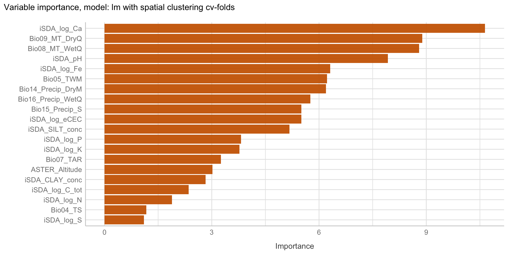
Figure 45: Variable importance plot, model: lm, resampling: spatial clustering cv-folds
Show code
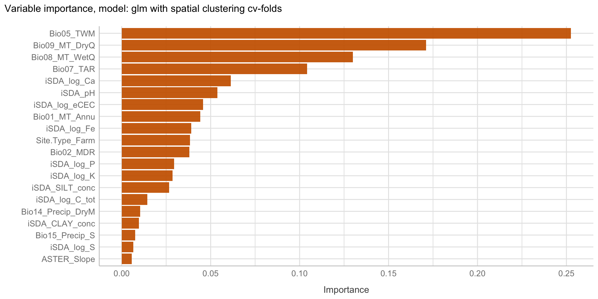
Figure 46: Variable importance plot, model: glm, resampling: spatial clustering cv-folds
Show code
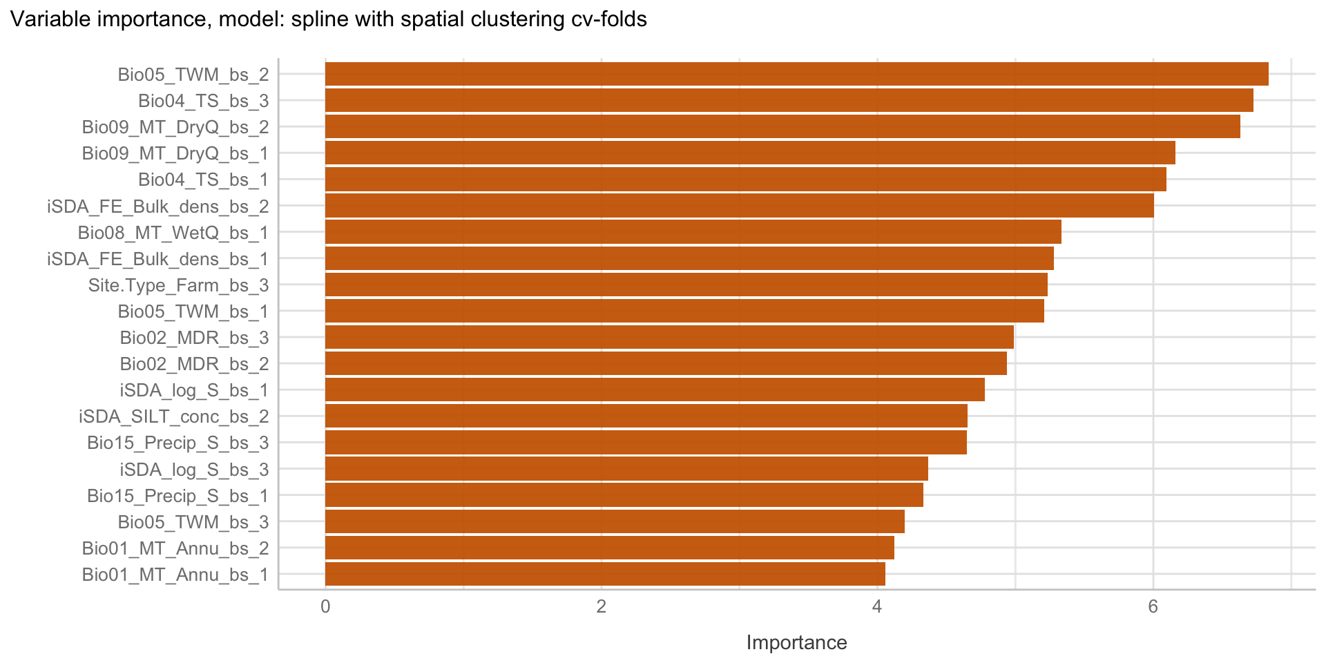
Figure 47: Variable importance plot, model: Spline, resampling: spatial clustering cv-folds
Show code
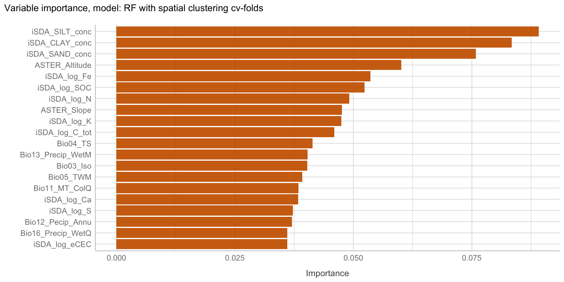
Figure 48: Variable importance plot, model: Random forest, resampling: spatial clustering cv-folds
Show code
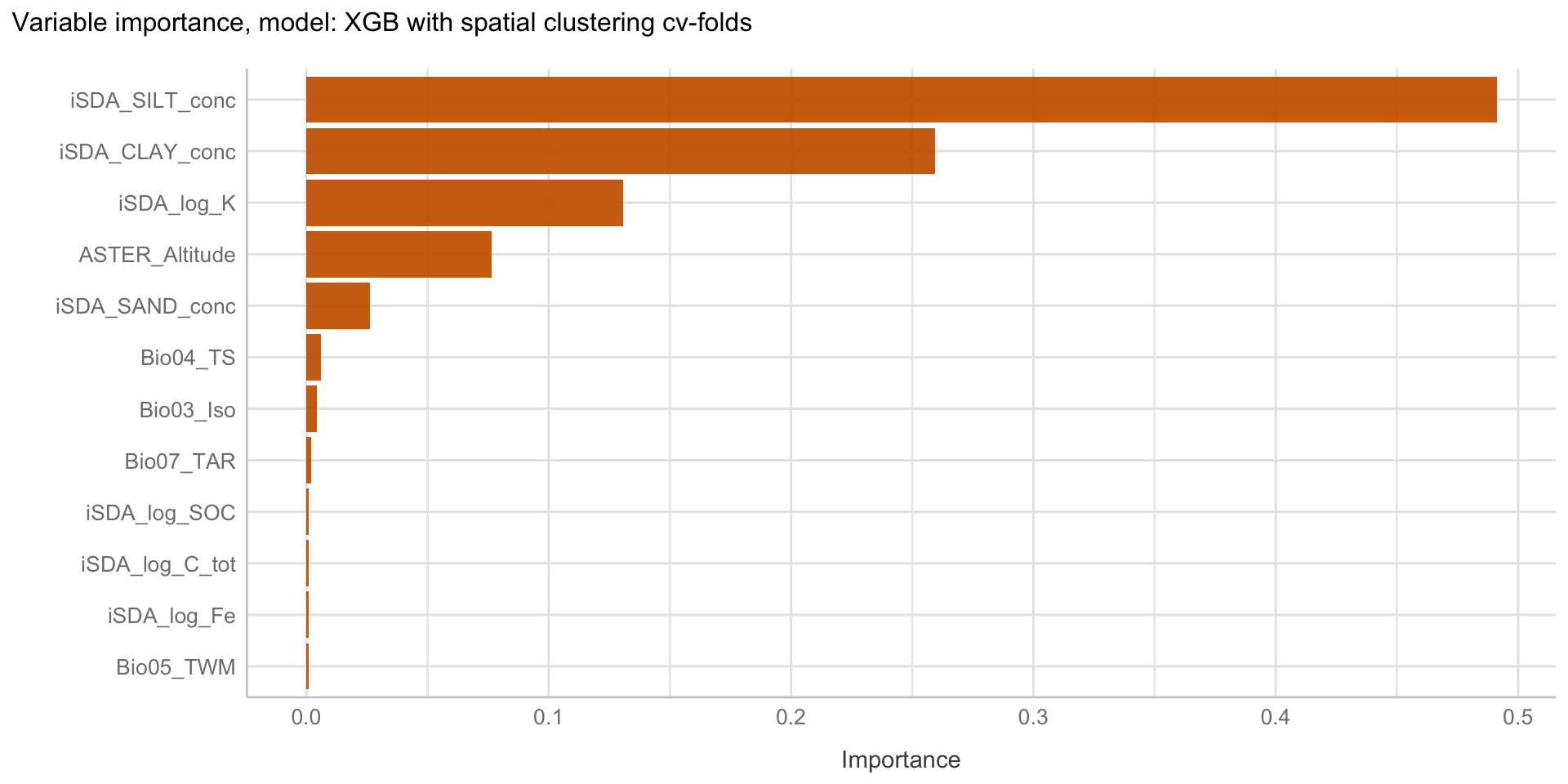
Figure 49: Variable importance plot, model: XGBoost, resampling: spatial clustering cv-folds
VIP for models with normal cv-folds

Figure 50: Variable importance plot, model: lm, resampling: Normal cv-folds

Figure 51: Variable importance plot, model: glm, resampling: Normal cv-folds
Show code
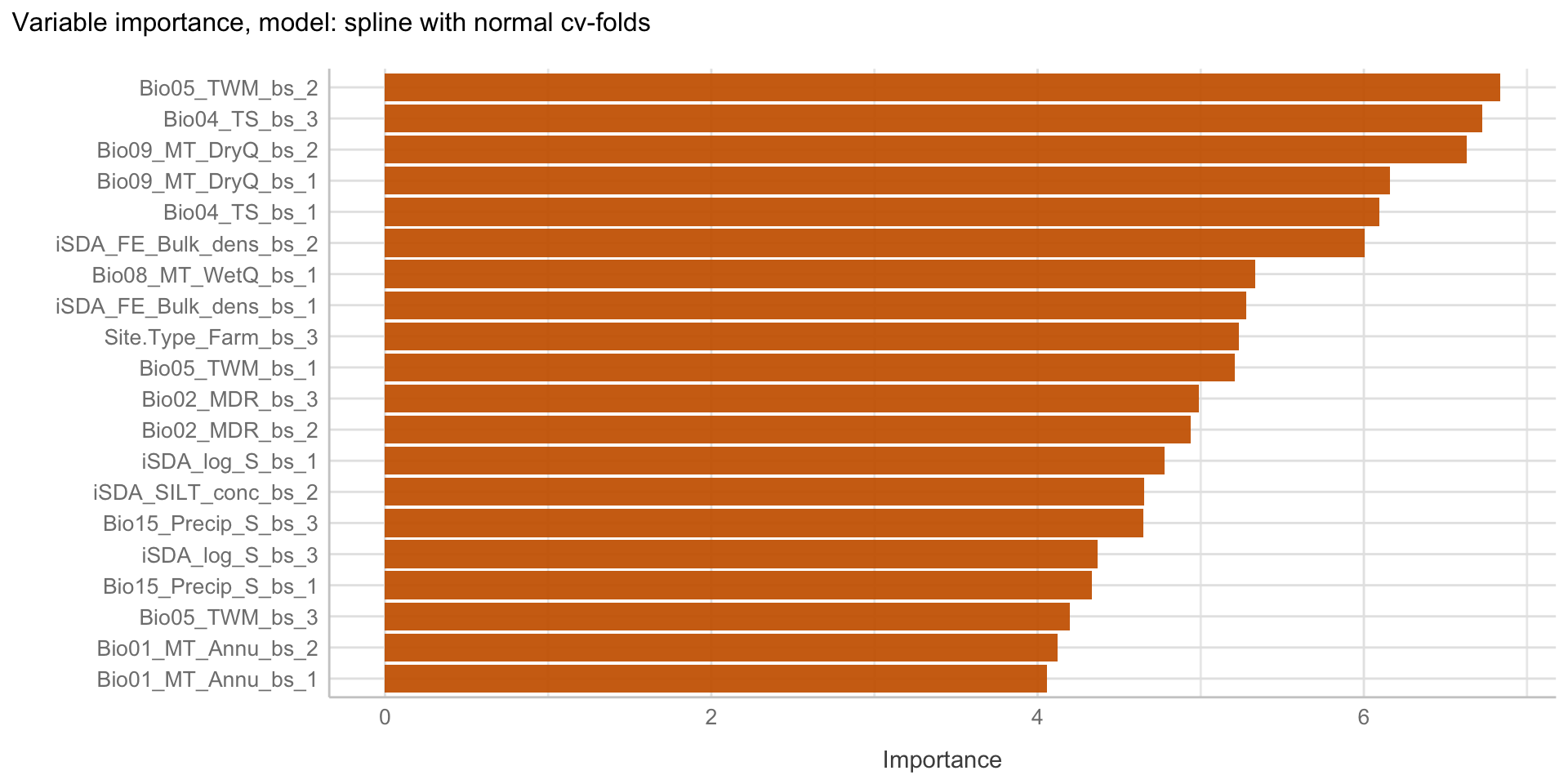
Figure 52: Variable importance plot, model: Spline, resampling: Normal cv-folds
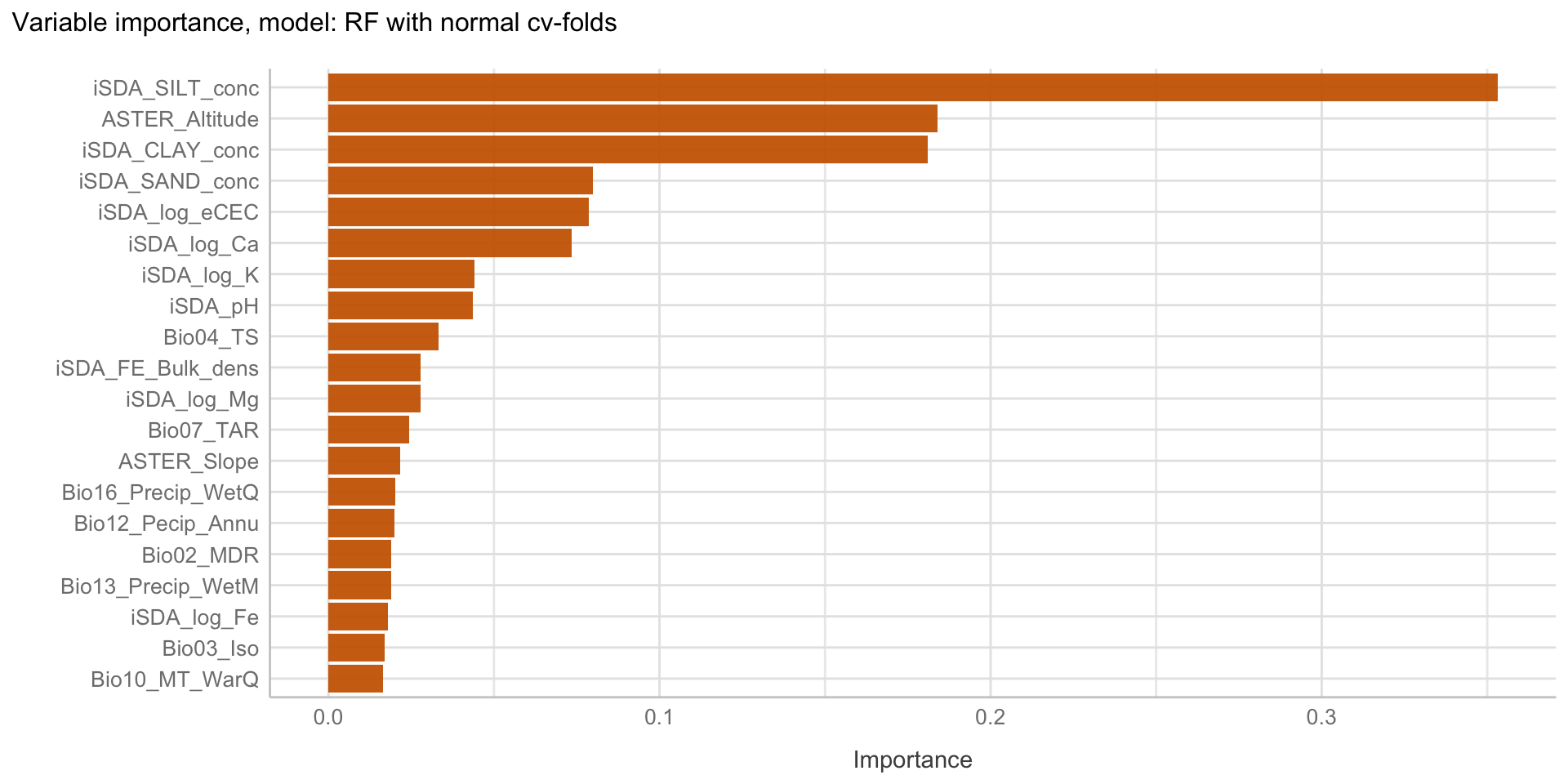
Figure 53: Variable importance plot, model: Random forest, resampling: Normal cv-folds
Show code
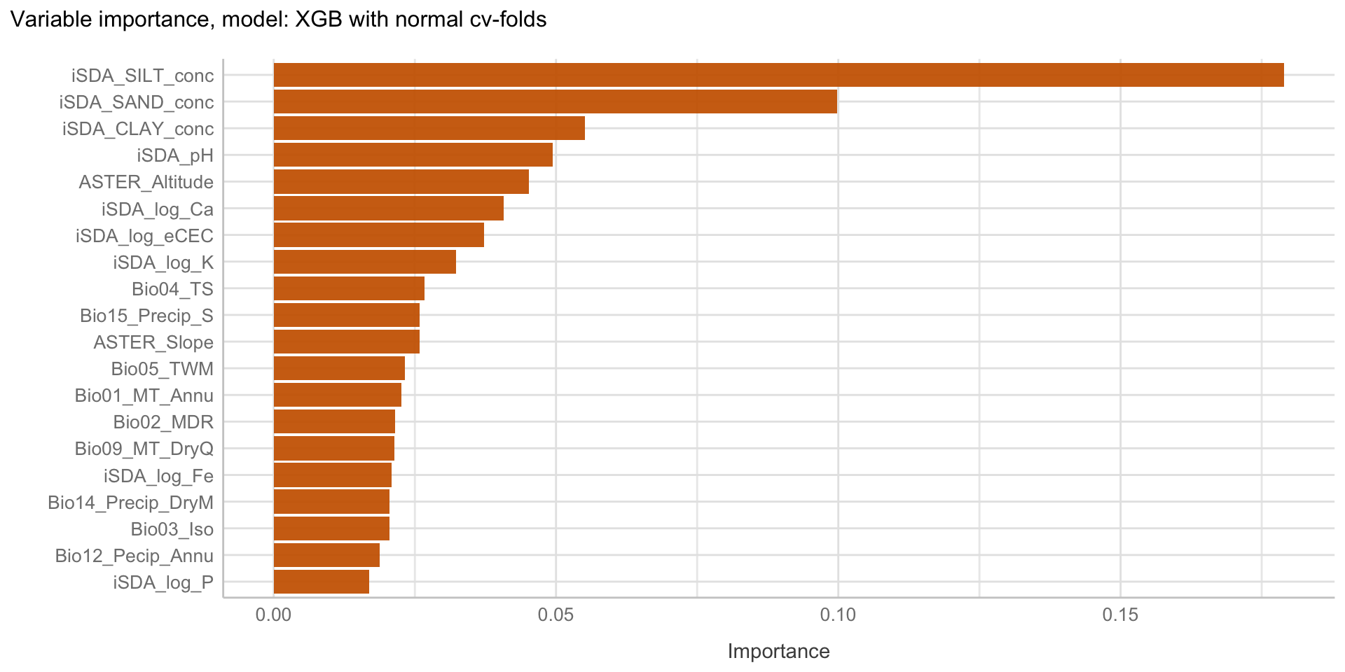
Figure 54: Variable importance plot, model: XGBoost, resampling: Normal cv-folds
Yardstick model evaluation
The yardstck package is part of the tidymodels meta-package and is made specifically to estimate how well models are working using tidy data principles. We are going to use the yardstick package functions to
##############################################################################################################
# Spatial k-fold cross validation
##############################################################################################################
# linear model (lm) --##--##--##--##--##--##--##--##--##--##--##--##--##--##--##--##--##--##--##--##--##--##--
# Prep the recipe in order to make the recipe ready to bake on the training and test data
lm_recipe_prepped <- prep(lm_recipe)
# Evaluate model on the training data ----------------------------------------------------------------------
lm_train_baked <- bake(lm_recipe_prepped, new_data = training(af.split))
lm_fit_spatcv_train_pred <- lm_final_model_spatcv %>% # fit the normal cv_folds model on all the training data
fit(formula = logRR ~ . ,data = lm_train_baked) %>% # predict logRR for the training data
predict(new_data = lm_train_baked) %>%
bind_cols(training(af.split))
# Evaluating model by measuring the accuracy of the model on training using `yardstick`
lm_spatcv_score_train <- lm_fit_spatcv_train_pred %>%
yardstick::metrics(logRR, .pred) %>%
mutate(.estimate = format(round(.estimate, 2), big.mark = ","))
# Evaluate model on the testing data -----------------------------------------------------------------------
lm_test_baked <- bake(lm_recipe_prepped, new_data = testing(af.split))
lm_fit_spatcv_test_pred <- lm_final_model_spatcv %>% # fit the normal cv_folds model on all the test data
fit(formula = logRR ~ ., data = lm_test_baked) %>% # use the training model fit to predict the test data
predict(new_data = lm_test_baked) %>%
bind_cols(testing(af.split))
# Evaluating model by measuring the accuracy of the model on testing data using `yardstick`
lm_spatcv_score_test <- lm_fit_spatcv_test_pred %>%
yardstick::metrics(logRR, .pred) %>%
mutate(.estimate = format(round(.estimate, 2), big.mark = ","))
# Visualising residuals
lm_spatcv_pred_resid <-
lm_fit_spatcv_test_pred %>%
arrange(.pred) %>%
mutate(residual_pct = (logRR - .pred) / .pred) %>%
select(.pred, residual_pct) %>%
ggplot(aes(x = .pred, y = residual_pct)) +
geom_point() +
xlab("Predicted logRR") +
ylab("Residual (%)")
# -----------------------------------------------
lm_spatcv_test_pred <-
predict(lm_final_model_spatcv %>%
fit(formula = logRR ~ .,
data = lm_test_baked),
new_data = lm_test_baked) %>%
bind_cols(af.test %>% dplyr::select(logRR))
saveRDS(lm_spatcv_test_pred, file = here::here("TidyMod_OUTPUT", "lm_spatcv_test_pred.RDS"))
# lm_spatcv_test_pred %>% rmse(logRR, .pred)
# Visualising predicted vs. observed logRR plot
lm_spatcv_test_pred_hexplot <-
lm_spatcv_test_pred %>%
ggplot(aes(x = logRR, y = .pred)) +
geom_abline(col = "black", lty = 1, size = 1) +
geom_hex(alpha = 0.8, bins = 50) +
geom_jitter(size = 0.8, width = 0.05, height = 0.05, shape = 3, alpha = 0.6) +
coord_fixed(ratio = 0.8) +
xlab("Observed logRR") +
ylab("Predicted logRR") +
scale_fill_viridis() +
ggtitle("Pred vs. obs logRR, model: lm with spatial clustering cv-fold") +
theme_lucid(plot.title.size = 10)
saveRDS(lm_spatcv_test_pred_hexplot, file = here::here("TidyMod_OUTPUT", "lm_spatcv_test_pred_hexplot.RDS"))
# Spline --##--##--##--##--##--##--##--##--##--##--##--##--##--##--##--##--##--##--##--##--##--##--##--
# Prep the recipe in order to make the recipe ready to bake on the training and test data
spline_recipe_prepped <- prep(spline_recipe)
# Evaluate model on the training data ----------------------------------------------------------------------
spline_train_baked <- bake(spline_recipe_prepped, new_data = training(af.split))
spline_fit_spatcv_train_pred <- spline_final_model_spatcv %>% # fit the normal cv_folds model on all the training data
fit(formula = logRR ~ . ,data = spline_train_baked) %>% # predict logRR for the training data
predict(new_data = spline_train_baked) %>%
bind_cols(training(af.split))
# Evaluating model by measuring the accuracy of the model on training using `yardstick`
spline_spatcv_score_train <- spline_fit_spatcv_train_pred %>%
yardstick::metrics(logRR, .pred) %>%
mutate(.estimate = format(round(.estimate, 2), big.mark = ","))
# Evaluate model on the testing data -----------------------------------------------------------------------
spline_test_baked <- bake(spline_recipe_prepped, new_data = testing(af.split))
spline_fit_spatcv_test_pred <- spline_final_model_spatcv %>% # fit the normal cv_folds model on all the test data
fit(formula = logRR ~ ., data = spline_test_baked) %>% # use the training model fit to predict the test data
predict(new_data = spline_test_baked) %>%
bind_cols(testing(af.split))
# Evaluating model by measuring the accuracy of the model on testing data using `yardstick`
spline_spatcv_score_test <- spline_fit_spatcv_test_pred %>%
yardstick::metrics(logRR, .pred) %>%
mutate(.estimate = format(round(.estimate, 2), big.mark = ","))
# Visualising residuals
spline_spatcv_pred_resid <-
spline_fit_spatcv_test_pred %>%
arrange(.pred) %>%
mutate(residual_pct = (logRR - .pred) / .pred) %>%
select(.pred, residual_pct) %>%
ggplot(aes(x = .pred, y = residual_pct)) +
geom_point() +
xlab("Predicted logRR") +
ylab("Residual (%)")
# -----------------------------------------------
spline_spatcv_test_pred <-
predict(spline_final_model_spatcv %>%
fit(formula = logRR ~ .,
data = spline_test_baked),
new_data = spline_test_baked) %>%
bind_cols(af.test %>% dplyr::select(logRR))
saveRDS(spline_spatcv_test_pred, file = here::here("TidyMod_OUTPUT", "spline_spatcv_test_pred.RDS"))
# spline_spatcv_test_pred %>% rmse(logRR, .pred)
spline_spatcv_test_pred_hexplot <-
spline_spatcv_test_pred %>%
ggplot(aes(x = logRR, y = .pred)) +
geom_abline(col = "black", lty = 1, size = 1) +
geom_hex(alpha = 0.8, bins = 50) +
geom_jitter(size = 0.8, width = 0.05, height = 0.05, shape = 3, alpha = 0.6) +
coord_fixed(ratio = 0.8) +
xlab("Observed logRR") +
ylab("Predicted logRR") +
scale_fill_viridis() +
ggtitle("Pred vs. obs logRR, model: Spline with spatial clustering cv-fold") +
theme_lucid(plot.title.size = 10)
saveRDS(spline_spatcv_test_pred_hexplot, file = here::here("TidyMod_OUTPUT", "spline_spatcv_test_pred_hexplot.RDS"))
# Random forest (RF) --##--##--##--##--##--##--##--##--##--##--##--##--##--##--##--##--##--##--##--##--##--##--
# Prep the recipe in order to make the recipe ready to bake on the training and test data
rf_xgboost_recipe_prepped <- prep(rf_xgboost_recipe)
# Evaluate model on the training data ----------------------------------------------------------------------
rf_xgboost_train_baked <- bake(rf_xgboost_recipe_prepped, new_data = training(af.split))
rf_fit_spatcv_train_pred <- rf_final_model_spatcv %>% # fit the normal cv_folds model on all the training data
fit(formula = logRR ~ . ,data = rf_xgboost_train_baked) %>% # predict logRR for the training data
predict(new_data = rf_xgboost_train_baked) %>%
bind_cols(training(af.split))
# Evaluating model by measuring the accuracy of the model on training using `yardstick`
rf_spatcv_score_train <- rf_fit_spatcv_train_pred %>%
yardstick::metrics(logRR, .pred) %>%
mutate(.estimate = format(round(.estimate, 2), big.mark = ","))
# Evaluate model on the testing data -----------------------------------------------------------------------
rf_xgboost_test_baked <- bake(rf_xgboost_recipe_prepped, new_data = testing(af.split))
rf_fit_spatcv_test_pred <- rf_final_model_spatcv %>% # fit the normal cv_folds model on all the test data
fit(formula = logRR ~ ., data = rf_xgboost_test_baked) %>% # use the training model fit to predict the test data
predict(new_data = rf_xgboost_test_baked) %>%
bind_cols(testing(af.split))
# Evaluating model by measuring the accuracy of the model on testing data using `yardstick`
rf_spatcv_score_test <- rf_fit_spatcv_test_pred %>%
yardstick::metrics(logRR, .pred) %>%
mutate(.estimate = format(round(.estimate, 2), big.mark = ","))
# Visualising residuals
rf_spatcv_pred_resid <-
rf_fit_spatcv_test_pred %>%
arrange(.pred) %>%
mutate(residual_pct = (logRR - .pred) / .pred) %>%
select(.pred, residual_pct) %>%
ggplot(aes(x = .pred, y = residual_pct)) +
geom_point() +
xlab("Predicted logRR") +
ylab("Residual (%)")
# -----------------------------------------------
rf_spatcv_test_pred <-
predict(rf_final_model_spatcv %>%
fit(formula = logRR ~ ., data = rf_xgboost_test_baked),
new_data = rf_xgboost_test_baked) %>%
bind_cols(af.test %>% dplyr::select(logRR))
# rf_spatcv_test_pred %>% rmse(logRR, .pred)
saveRDS(rf_spatcv_test_pred, file = here::here("TidyMod_OUTPUT", "rf_spatcv_test_pred.RDS"))
rf_spatcv_test_pred <- readRDS(file = here::here("TidyMod_OUTPUT", "rf_spatcv_test_pred.RDS"))
rf_spatcv_test_pred_hexplot <-
rf_spatcv_test_pred %>%
ggplot(aes(x = logRR, y = .pred)) +
geom_hex(alpha = 0.9, bins = 35) +
#geom_jitter(size = 0.5, width = 0.05, height = 0.05, shape = 3, alpha = 0.3) +
coord_obs_pred(ratio = 1.2) +
geom_abline(col = "black", lty = 1, size = 1) +
# coord_fixed(ratio = 1) +
xlab("Observed logRR") +
ylab("Predicted logRR") +
scale_fill_viridis_c(direction = -1, option = "D") +
ggtitle("Pred vs. obs logRR, model: RF with spatial clustering cv-fold") +
theme_lucid(plot.title.size = 10)
saveRDS(rf_spatcv_test_pred_hexplot, file = here::here("TidyMod_OUTPUT", "rf_spatcv_test_pred_hexplot.RDS"))
# XGBoost (xgb) --##--##--##--##--##--##--##--##--##--##--##--##--##--##--##--##--##--##--##--##--##--##--
xgb_fit_spatcv_train_pred <- xgb_final_model_spatcv %>% # fit the normal cv_folds model on all the training data
fit(formula = logRR ~ . ,data = rf_xgboost_train_baked) %>% # predict logRR for the training data
predict(new_data = rf_xgboost_train_baked) %>%
bind_cols(training(af.split))
# Evaluating model by measuring the accuracy of the model on training using `yardstick`
xgb_spatcv_score_train <- xgb_fit_spatcv_train_pred %>%
yardstick::metrics(logRR, .pred) %>%
mutate(.estimate = format(round(.estimate, 2), big.mark = ","))
# Evaluate model on the testing data -----------------------------------------------------------------------
xgb_fit_spatcv_test_pred <- xgb_final_model_spatcv %>% # fit the normal cv_folds model on all the test data
fit(formula = logRR ~ ., data = rf_xgboost_test_baked) %>% # use the training model fit to predict the test data
predict(new_data = rf_xgboost_test_baked) %>%
bind_cols(testing(af.split))
# Evaluating model by measuring the accuracy of the model on testing data using `yardstick`
xgb_spatcv_score_test <- xgb_fit_spatcv_test_pred %>%
yardstick::metrics(logRR, .pred) %>%
mutate(.estimate = format(round(.estimate, 2), big.mark = ","))
# Visualising residuals
xgb_spatcv_pred_resid <-
xgb_fit_spatcv_test_pred %>%
arrange(.pred) %>%
mutate(residual_pct = (logRR - .pred) / .pred) %>%
select(.pred, residual_pct) %>%
ggplot(aes(x = .pred, y = residual_pct)) +
geom_point() +
xlab("Predicted logRR") +
ylab("Residual (%)")
# -----------------------------------------------
xgb_spatcv_test_pred <-
predict(xgb_final_model_spatcv %>%
fit(formula = logRR ~ ., data = rf_xgboost_test_baked),
new_data = rf_xgboost_test_baked) %>%
bind_cols(af.test %>% dplyr::select(logRR))
# xgb_spatcv_test_pred %>% rmse(logRR, .pred)
saveRDS(xgb_spatcv_test_pred, file = here::here("TidyMod_OUTPUT", "xgb_spatcv_test_pred.RDS"))
xgb_spatcv_test_pred_hexplot <-
xgb_spatcv_test_pred %>%
ggplot(aes(x = logRR, y = .pred)) +
geom_abline(col = "black", lty = 1, size = 1) +
geom_hex(alpha = 0.8, bins = 50) +
geom_jitter(size = 0.8, width = 0.05, height = 0.05, shape = 3, alpha = 0.6) +
coord_fixed(ratio = 10) + # <- NOTICE the change in plot coord because something wiered is happening with xgb spatcv
xlab("Observed logRR") +
ylab("Predicted logRR") +
scale_fill_viridis() +
ggtitle("Pred vs. obs logRR, model: xgb with spatial clustering cv-fold") +
theme_lucid(plot.title.size = 10)
saveRDS(xgb_spatcv_test_pred_hexplot, file = here::here("TidyMod_OUTPUT", "xgb_spatcv_test_pred_hexplot.RDS"))
##############################################################################################################
# Normal (random) k-fold cross validation (CV-fold)
##############################################################################################################
# linear model (lm) --##--##--##--##--##--##--##--##--##--##--##--##--##--##--##--##--##--##--##--##--##--##--
# Prep the recipe in order to make the recipe ready to bake on the training and test data
lm_recipe_prepped <- prep(lm_recipe)
# Evaluate model on the training data ----------------------------------------------------------------------
lm_train_baked <- bake(lm_recipe_prepped, new_data = training(af.split))
lm_fit_cv_train_pred <- lm_final_model_cv %>% # fit the normal cv_folds model on all the training data
fit(formula = logRR ~ . ,data = lm_train_baked) %>% # predict logRR for the training data
predict(new_data = lm_train_baked) %>%
bind_cols(training(af.split))
# Evaluating model by measuring the accuracy of the model on training using `yardstick`
lm_cv_score_train <- lm_fit_cv_train_pred %>%
yardstick::metrics(logRR, .pred) %>%
mutate(.estimate = format(round(.estimate, 2), big.mark = ","))
# Evaluate model on the testing data -----------------------------------------------------------------------
lm_test_baked <- bake(lm_recipe_prepped, new_data = testing(af.split))
lm_fit_cv_test_pred <- lm_final_model_cv %>% # fit the normal cv_folds model on all the test data
fit(formula = logRR ~ ., data = lm_test_baked) %>% # use the training model fit to predict the test data
predict(new_data = lm_test_baked) %>%
bind_cols(testing(af.split))
# Evaluating model by measuring the accuracy of the model on testing data using `yardstick`
lm_cv_score_test <- lm_fit_cv_test_pred %>%
yardstick::metrics(logRR, .pred) %>%
mutate(.estimate = format(round(.estimate, 2), big.mark = ","))
# Visualising residuals
lm_cv_pred_resid <-
lm_fit_cv_test_pred %>%
arrange(.pred) %>%
mutate(residual_pct = (logRR - .pred) / .pred) %>%
select(.pred, residual_pct) %>%
ggplot(aes(x = .pred, y = residual_pct)) +
geom_point() +
xlab("Predicted logRR") +
ylab("Residual (%)")
# -----------------------------------------------
lm_cv_test_pred <-
predict(lm_final_model_cv %>%
fit(formula = logRR ~ .,
data = lm_test_baked),
new_data = lm_test_baked) %>%
bind_cols(af.test %>% dplyr::select(logRR))
# lm_cv_test_pred %>% rmse(logRR, .pred)
saveRDS(lm_cv_test_pred, file = here::here("TidyMod_OUTPUT", "lm_cv_test_pred.RDS"))
lm_cv_test_pred_hexplot <-
lm_cv_test_pred %>%
ggplot(aes(x = logRR, y = .pred)) +
geom_abline(col = "black", lty = 1, size = 1) +
geom_hex(alpha = 0.8, bins = 50) +
geom_jitter(size = 0.8, width = 0.05, height = 0.05, shape = 3, alpha = 0.6) +
coord_fixed(ratio = 0.8) +
xlab("Observed logRR") +
ylab("Predicted logRR") +
scale_fill_viridis() +
ggtitle("Pred vs. obs logRR, model: lm with normal cv-fold") +
theme_lucid(plot.title.size = 10)
saveRDS(lm_cv_test_pred_hexplot, file = here::here("TidyMod_OUTPUT", "lm_cv_test_pred_hexplot.RDS"))
# Spline --##--##--##--##--##--##--##--##--##--##--##--##--##--##--##--##--##--##--##--##--##--##--##--
# Prep the recipe in order to make the recipe ready to bake on the training and test data
spline_recipe_prepped <- prep(spline_recipe)
# Evaluate model on the training data ----------------------------------------------------------------------
spline_train_baked <- bake(spline_recipe_prepped, new_data = training(af.split))
spline_fit_cv_train_pred <- spline_final_model_cv %>% # fit the normal cv_folds model on all the training data
fit(formula = logRR ~ . ,data = spline_train_baked) %>% # predict logRR for the training data
predict(new_data = spline_train_baked) %>%
bind_cols(training(af.split))
# Evaluating model by measuring the accuracy of the model on training using `yardstick`
spline_cv_score_train <- spline_fit_cv_train_pred %>%
yardstick::metrics(logRR, .pred) %>%
mutate(.estimate = format(round(.estimate, 2), big.mark = ","))
# Evaluate model on the testing data -----------------------------------------------------------------------
spline_test_baked <- bake(spline_recipe_prepped, new_data = testing(af.split))
spline_fit_cv_test_pred <- spline_final_model_cv %>% # fit the normal cv_folds model on all the test data
fit(formula = logRR ~ ., data = spline_test_baked) %>% # use the training model fit to predict the test data
predict(new_data = spline_test_baked) %>%
bind_cols(testing(af.split))
# Evaluating model by measuring the accuracy of the model on testing data using `yardstick`
spline_cv_score_test <- spline_fit_cv_test_pred %>%
yardstick::metrics(logRR, .pred) %>%
mutate(.estimate = format(round(.estimate, 2), big.mark = ","))
# Visualising residuals
spline_cv_pred_resid <-
spline_fit_cv_test_pred %>%
arrange(.pred) %>%
mutate(residual_pct = (logRR - .pred) / .pred) %>%
select(.pred, residual_pct) %>%
ggplot(aes(x = .pred, y = residual_pct)) +
geom_point() +
xlab("Predicted logRR") +
ylab("Residual (%)")
# -----------------------------------------------
spline_cv_test_pred <-
predict(spline_final_model_cv %>%
fit(formula = logRR ~ .,
data = spline_test_baked),
new_data = spline_test_baked) %>%
bind_cols(af.test %>% dplyr::select(logRR))
# spline_cv_test_pred %>% rmse(logRR, .pred)
saveRDS(spline_cv_test_pred, file = here::here("TidyMod_OUTPUT", "spline_cv_test_pred.RDS"))
spline_cv_test_pred_hexplot <-
spline_cv_test_pred %>%
ggplot(aes(x = logRR, y = .pred)) +
geom_abline(col = "black", lty = 1, size = 1) +
geom_hex(alpha = 0.8, bins = 50) +
geom_jitter(size = 0.8, width = 0.05, height = 0.05, shape = 3, alpha = 0.6) +
coord_fixed(ratio = 0.8) +
xlab("Observed logRR") +
ylab("Predicted logRR") +
scale_fill_viridis() +
ggtitle("Pred vs. obs logRR, model: Spline with normal cv-fold") +
theme_lucid(plot.title.size = 10)
saveRDS(spline_cv_test_pred_hexplot, file = here::here("TidyMod_OUTPUT", "spline_cv_test_pred_hexplot.RDS"))
# Random forest (RF) --##--##--##--##--##--##--##--##--##--##--##--##--##--##--##--##--##--##--##--##--##--##--
# Prep the recipe in order to make the recipe ready to bake on the training and test data
rf_xgboost_recipe_prepped <- prep(rf_xgboost_recipe)
# Evaluate model on the training data ----------------------------------------------------------------------
rf_xgboost_train_baked <- bake(rf_xgboost_recipe_prepped, new_data = training(af.split))
rf_fit_cv_train_pred <- rf_final_model_cv %>% # fit the normal cv_folds model on all the training data
fit(formula = logRR ~ . ,data = rf_xgboost_train_baked) %>% # predict logRR for the training data
predict(new_data = rf_xgboost_train_baked) %>%
bind_cols(training(af.split))
# Evaluating model by measuring the accuracy of the model on training using `yardstick`
rf_cv_score_train <- rf_fit_cv_train_pred %>%
yardstick::metrics(logRR, .pred) %>%
mutate(.estimate = format(round(.estimate, 2), big.mark = ","))
# Evaluate model on the testing data -----------------------------------------------------------------------
rf_xgboost_test_baked <- bake(rf_xgboost_recipe_prepped, new_data = testing(af.split))
rf_fit_cv_test_pred <- rf_final_model_cv %>% # fit the normal cv_folds model on all the test data
fit(formula = logRR ~ ., data = rf_xgboost_test_baked) %>% # use the training model fit to predict the test data
predict(new_data = rf_xgboost_test_baked) %>%
bind_cols(testing(af.split))
# Evaluating model by measuring the accuracy of the model on testing data using `yardstick`
rf_cv_score_test <- rf_fit_cv_test_pred %>%
yardstick::metrics(logRR, .pred) %>%
mutate(.estimate = format(round(.estimate, 2), big.mark = ","))
# Visualising residuals
rf_cv_pred_resid <-
rf_fit_cv_test_pred %>%
arrange(.pred) %>%
mutate(residual_pct = (logRR - .pred) / .pred) %>%
select(.pred, residual_pct) %>%
ggplot(aes(x = .pred, y = residual_pct)) +
geom_point() +
xlab("Predicted logRR") +
ylab("Residual (%)")
# -----------------------------------------------
rf_cv_test_pred <-
predict(rf_final_model_cv %>%
fit(formula = logRR ~ ., data = rf_xgboost_test_baked),
new_data = rf_xgboost_test_baked) %>%
bind_cols(af.test %>% dplyr::select(logRR))
# rf_cv_test_pred %>% rmse(logRR, .pred)
saveRDS(rf_cv_test_pred, file = here::here("TidyMod_OUTPUT", "rf_cv_test_pred.RDS"))
rf_cv_test_pred_hexplot <-
rf_cv_test_pred %>%
ggplot(aes(x = logRR, y = .pred)) +
geom_abline(col = "black", lty = 1, size = 1) +
geom_hex(alpha = 0.8, bins = 50) +
geom_jitter(size = 0.8, width = 0.05, height = 0.05, shape = 3, alpha = 0.6) +
coord_fixed(ratio = 0.8) +
xlab("Observed logRR") +
ylab("Predicted logRR") +
scale_fill_viridis() +
ggtitle("Pred vs. obs logRR, model: RF with normal cv-fold") +
theme_lucid(plot.title.size = 10)
saveRDS(rf_cv_test_pred_hexplot, file = here::here("TidyMod_OUTPUT", "rf_cv_test_pred_hexplot.RDS"))
# XGBoost (xgb) --##--##--##--##--##--##--##--##--##--##--##--##--##--##--##--##--##--##--##--##--##--##--
xgb_fit_cv_train_pred <- xgb_final_model_cv %>% # fit the normal cv_folds model on all the training data
fit(formula = logRR ~ . ,data = rf_xgboost_train_baked) %>% # predict logRR for the training data
predict(new_data = rf_xgboost_train_baked) %>%
bind_cols(training(af.split))
# Evaluating model by measuring the accuracy of the model on training using `yardstick`
xgb_cv_score_train <- xgb_fit_cv_train_pred %>%
yardstick::metrics(logRR, .pred) %>%
mutate(.estimate = format(round(.estimate, 2), big.mark = ","))
# Evaluate model on the testing data -----------------------------------------------------------------------
xgb_fit_cv_test_pred <- xgb_final_model_cv %>% # fit the normal cv_folds model on all the test data
fit(formula = logRR ~ ., data = rf_xgboost_test_baked) %>% # use the training model fit to predict the test data
predict(new_data = rf_xgboost_test_baked) %>%
bind_cols(testing(af.split))
# Evaluating model by measuring the accuracy of the model on testing data using `yardstick`
xgb_cv_score_test <- xgb_fit_cv_test_pred %>%
yardstick::metrics(logRR, .pred) %>%
mutate(.estimate = format(round(.estimate, 2), big.mark = ","))
# Visualising residuals
xgb_cv_pred_resid <-
xgb_fit_cv_test_pred %>%
arrange(.pred) %>%
mutate(residual_pct = (logRR - .pred) / .pred) %>%
select(.pred, residual_pct) %>%
ggplot(aes(x = .pred, y = residual_pct)) +
geom_point() +
xlab("Predicted logRR") +
ylab("Residual (%)")
# -----------------------------------------------
xgb_cv_test_pred <-
predict(xgb_final_model_cv %>%
fit(formula = logRR ~ ., data = rf_xgboost_test_baked),
new_data = rf_xgboost_test_baked) %>%
bind_cols(af.test %>% dplyr::select(logRR))
# xgb_cv_test_pred %>% rmse(logRR, .pred)
saveRDS(xgb_cv_test_pred, file = here::here("TidyMod_OUTPUT", "xgb_cv_test_pred.RDS"))
xgb_cv_test_pred_hexplot <-
xgb_cv_test_pred %>%
ggplot(aes(x = logRR, y = .pred)) +
geom_abline(col = "black", lty = 1, size = 1) +
geom_hex(alpha = 0.8, bins = 50) +
geom_jitter(size = 0.8, width = 0.05, height = 0.05, shape = 3, alpha = 0.6) +
coord_fixed(ratio = 0.8) +
xlab("Observed logRR") +
ylab("Predicted logRR") +
scale_fill_viridis() +
ggtitle("Pred vs. obs logRR, model: xgb with spatial clustering cv-fold") +
theme_lucid(plot.title.size = 10)
saveRDS(xgb_cv_test_pred_hexplot, file = here::here("TidyMod_OUTPUT", "xgb_cv_test_pred_hexplot.RDS"))
# -----
# Warning in predict.lm(object = object$fit, newdata = new_data, type = "response") :
# prediction from a rank-deficient fit may be misleading
# Warning in predict.lm(object = object$fit, newdata = new_data, type = "response") :
# prediction from a rank-deficient fit may be misleading
# Warning in predict.lm(object = object$fit, newdata = new_data, type = "response") :
# prediction from a rank-deficient fit may be misleading
# Adding missing grouping variables: `ERA_Agroforestry`
# Warning in predict.lm(object = object$fit, newdata = new_data, type = "response") :
# prediction from a rank-deficient fit may be misleading
# Warning in predict.lm(object = object$fit, newdata = new_data, type = "response") :
# prediction from a rank-deficient fit may be misleading
# Warning in predict.lm(object = object$fit, newdata = new_data, type = "response") :
# prediction from a rank-deficient fit may be misleading
# Adding missing grouping variables: `ERA_Agroforestry`
# Adding missing grouping variables: `ERA_Agroforestry`
# Warning in predict.lm(object = object$fit, newdata = new_data, type = "response") :
# prediction from a rank-deficient fit may be misleading
# Warning in predict.lm(object = object$fit, newdata = new_data, type = "response") :
# prediction from a rank-deficient fit may be misleading
# Warning in predict.lm(object = object$fit, newdata = new_data, type = "response") :
# prediction from a rank-deficient fit may be misleading
# Adding missing grouping variables: `ERA_Agroforestry`
# Adding missing grouping variables: `ERA_Agroforestry`
# -----
Show code
##############################################################################################################
# Spatial clustering cv-fold
lm_spatcv_test_pred %>% rmse(logRR, .pred)
spline_spatcv_test_pred %>% rmse(logRR, .pred)
rf_spatcv_test_pred %>% rmse(logRR, .pred)
xgb_spatcv_test_pred %>% rmse(logRR, .pred)
##############################################################################################################
# Normal (random) cv-fold
lm_cv_test_pred %>% rmse(logRR, .pred)
spline_cv_test_pred %>% rmse(logRR, .pred)
rf_cv_test_pred %>% rmse(logRR, .pred)
xgb_cv_test_pred %>% rmse(logRR, .pred)
##############################################################################################################
# Loading data
lm_spatcv_test_pred <- readRDS(file = here::here("TidyMod_OUTPUT", "lm_spatcv_test_pred.RDS"))
spline_spatcv_test_pred <- readRDS(file = here::here("TidyMod_OUTPUT", "spline_spatcv_test_pred.RDS"))
rf_spatcv_test_pred <- readRDS(file = here::here("TidyMod_OUTPUT", "rf_spatcv_test_pred.RDS"))
xgb_spatcv_test_pred <- readRDS(file = here::here("TidyMod_OUTPUT", "xgb_spatcv_test_pred.RDS"))
lm_cv_test_pred <- readRDS(file = here::here("TidyMod_OUTPUT", "lm_cv_test_pred.RDS"))
spline_cv_test_pred <- readRDS(file = here::here("TidyMod_OUTPUT", "spline_cv_test_pred.RDS"))
rf_cv_test_pred <- readRDS(file = here::here("TidyMod_OUTPUT", "rf_cv_test_pred.RDS"))
xgb_cv_test_pred <- readRDS(file = here::here("TidyMod_OUTPUT", "xgb_cv_test_pred.RDS"))
# Metrics (yardstick metrics set)
metric_set <- yardstick::metric_set(rmse, mae, ccc, rsq, rpd, rpiq)
##############################################################################################################
# Spatial clustering cv-fold
lm_spatcv_metric <- lm_spatcv_test_pred %>% metric_set(logRR, .pred)
spline_spatcv_metric <- spline_spatcv_test_pred %>% metric_set(logRR, .pred)
rf_spatcv_metric <- rf_spatcv_test_pred %>% metric_set(logRR, .pred)
xgb_spatcv_metric <- xgb_spatcv_test_pred %>% metric_set(logRR, .pred)
models_spatcv_metrics <-
lm_spatcv_metric %>%
left_join(spline_spatcv_metric, by = c(".estimator", ".metric")) %>%
left_join(rf_spatcv_metric, by = c(".estimator", ".metric")) %>%
left_join(xgb_spatcv_metric, by = c(".estimator", ".metric")) %>%
rename(lm_spatcv_est = ".estimate.x",
spline_spatcv_est = ".estimate.y",
rf_spatcv_est = ".estimate.x.x",
xgb_spatcv_est = ".estimate.y.y") %>%
dplyr::select(!.estimator)
##############################################################################################################
# Normal (random) cv-fold
lm_cv_metric <- lm_cv_test_pred %>% metric_set(logRR, .pred)
spline_cv_metrics <- spline_cv_test_pred %>% metric_set(logRR, .pred)
rf_cv_metrics <- rf_cv_test_pred %>% metric_set(logRR, .pred)
xgb_cv_metrics <- xgb_cv_test_pred %>% metric_set(logRR, .pred)
models_cv_metrics <-
lm_cv_metric %>%
left_join(spline_cv_metrics, by = c(".estimator", ".metric")) %>%
left_join(rf_cv_metrics, by = c(".estimator", ".metric")) %>%
left_join(xgb_cv_metrics, by = c(".estimator", ".metric")) %>%
rename(lm_cv_est = ".estimate.x",
spline_cv_est = ".estimate.y",
rf_cv_est = ".estimate.x.x",
xgb_cv_est = ".estimate.y.y") %>%
dplyr::select(!.estimator)
# -----------------------------------------------------------------------------------------------------------
models_metrics <-
models_spatcv_metrics %>%
left_join(models_cv_metrics, by = ".metric")
models_metrics
# A tibble: 6 × 9
.metric lm_spatcv_est spline_spatcv_est rf_spatcv_est xgb_spatcv_est
<chr> <dbl> <dbl> <dbl> <dbl>
1 rmse 0.505 0.469 0.505 0.736
2 mae 0.364 0.322 0.367 0.556
3 ccc 0.698 0.750 0.681 0.0399
4 rsq 0.537 0.601 0.541 0.241
5 rpd 1.47 1.58 1.47 1.01
6 rpiq 1.53 1.65 1.53 1.05
# … with 4 more variables: lm_cv_est <dbl>, spline_cv_est <dbl>,
# rf_cv_est <dbl>, xgb_cv_est <dbl>Evaluating all models on model metrics
Show code
##############################################################################################################
# Spatial k-fold cross validation
##############################################################################################################
# TRAINING DATA
# Metrics for all the models on the training data ---------------------- ---------------------- ----------------------
lm_spatcv_train_pred_metric_table <-
lm_fit_spatcv_train_pred %>% metric_set(logRR, .pred) %>%
mutate(model_and_cv_type = "lm_spatcv") %>%
select(-.estimator) %>%
relocate(model_and_cv_type, .metric, .estimate)
spline_spatcv_train_pred_metric_table <-
spline_fit_spatcv_train_pred %>% metric_set(logRR, .pred) %>%
mutate(model_and_cv_type = "spline_spatcv") %>%
select(-.estimator) %>%
relocate(model_and_cv_type, .metric, .estimate)
rf_spatcv_train_pred_metric_table <-
rf_fit_spatcv_train_pred %>% metric_set(logRR, .pred) %>%
mutate(model_and_cv_type = "rf_spatcv") %>%
select(-.estimator) %>%
relocate(model_and_cv_type, .metric, .estimate)
xgb_spatcv_train_pred_metric_table <-
xgb_fit_spatcv_train_pred %>% metric_set(logRR, .pred) %>%
mutate(model_and_cv_type = "xgb_spatcv") %>%
select(-.estimator) %>%
relocate(model_and_cv_type, .metric, .estimate)
all_models_spatcv_training_data_metric_rmse <- bind_rows(lm_spatcv_train_pred_metric_table,
spline_spatcv_train_pred_metric_table,
rf_spatcv_train_pred_metric_table,
xgb_spatcv_train_pred_metric_table) %>%
dplyr::filter(.metric == "rmse") %>%
dplyr::arrange(-desc(.estimate))
all_models_spatcv_training_data_metric_rmse
# Saving data
saveRDS(all_models_spatcv_training_data_metric_rmse, here::here("TidyMod_OUTPUT", "all_models_spatcv_training_data_metric_rmse.RDS"))
# TESTING DATA
# Metrics for all the models on the testing data ---------------------- ---------------------- ----------------------
lm_spatcv_test_pred_metric_table <-
lm_fit_spatcv_test_pred %>% metric_set(logRR, .pred) %>%
mutate(model_and_cv_type = "lm_spatcv") %>%
select(-.estimator) %>%
relocate(model_and_cv_type, .metric, .estimate)
spline_spatcv_test_pred_metric_table <-
spline_fit_spatcv_test_pred %>% metric_set(logRR, .pred) %>%
mutate(model_and_cv_type = "spline_spatcv") %>%
select(-.estimator) %>%
relocate(model_and_cv_type, .metric, .estimate)
rf_spatcv_test_pred_metric_table <-
rf_fit_spatcv_test_pred %>% metric_set(logRR, .pred) %>%
mutate(model_and_cv_type = "rf_spatcv") %>%
select(-.estimator) %>%
relocate(model_and_cv_type, .metric, .estimate)
xgb_spatcv_test_pred_metric_table <-
xgb_fit_spatcv_test_pred %>% metric_set(logRR, .pred) %>%
mutate(model_and_cv_type = "xgb_spatcv") %>%
select(-.estimator) %>%
relocate(model_and_cv_type, .metric, .estimate)
all_models_spatcv_testing_data_metric_rmse <- bind_rows(lm_spatcv_test_pred_metric_table,
spline_spatcv_test_pred_metric_table,
rf_spatcv_test_pred_metric_table,
xgb_spatcv_test_pred_metric_table) %>%
dplyr::filter(.metric == "rmse") %>%
dplyr::arrange(-desc(.estimate))
all_models_spatcv_testing_data_metric_rmse
# Saving data
saveRDS(all_models_spatcv_testing_data_metric_rmse, here::here("TidyMod_OUTPUT", "all_models_spatcv_testing_data_metric_rmse.RDS"))
##############################################################################################################
# Normal (random) k-fold cross validation (CV-fold)
##############################################################################################################
# TRAINING DATA
# Metrics for all the models on the training data ---------------------- ---------------------- ----------------------
lm_cv_train_pred_metric_table <-
lm_fit_cv_train_pred %>% metric_set(logRR, .pred) %>%
mutate(model_and_cv_type = "lm_cv") %>%
select(-.estimator) %>%
relocate(model_and_cv_type, .metric, .estimate)
spline_cv_train_pred_metric_table <-
spline_fit_cv_train_pred %>% metric_set(logRR, .pred) %>%
mutate(model_and_cv_type = "spline_cv") %>%
select(-.estimator) %>%
relocate(model_and_cv_type, .metric, .estimate)
rf_cv_train_pred_metric_table <-
rf_fit_cv_train_pred %>% metric_set(logRR, .pred) %>%
mutate(model_and_cv_type = "rf_cv") %>%
select(-.estimator) %>%
relocate(model_and_cv_type, .metric, .estimate)
xgb_cv_train_pred_metric_table <-
xgb_fit_cv_train_pred %>% metric_set(logRR, .pred) %>%
mutate(model_and_cv_type = "xgb_cv") %>%
select(-.estimator) %>%
relocate(model_and_cv_type, .metric, .estimate)
all_models_cv_training_data_metric_rmse <- bind_rows(lm_cv_train_pred_metric_table,
spline_cv_train_pred_metric_table,
rf_cv_train_pred_metric_table,
xgb_cv_train_pred_metric_table) %>%
dplyr::filter(.metric == "rmse") %>%
dplyr::arrange(-desc(.estimate))
all_models_cv_training_data_metric_rmse
# Saving data
saveRDS(all_models_cv_training_data_metric_rmse, here::here("TidyMod_OUTPUT", "all_models_cv_training_data_metric_rmse.RDS"))
# TESTING DATA
# Metrics for all the models on the testing data ---------------------- ---------------------- ----------------------
lm_cv_test_pred_metric_table <-
lm_fit_cv_test_pred %>% metric_set(logRR, .pred) %>%
mutate(model_and_cv_type = "lm_cv") %>%
select(-.estimator) %>%
relocate(model_and_cv_type, .metric, .estimate)
spline_cv_test_pred_metric_table <-
spline_fit_cv_test_pred %>% metric_set(logRR, .pred) %>%
mutate(model_and_cv_type = "spline_cv") %>%
select(-.estimator) %>%
relocate(model_and_cv_type, .metric, .estimate)
rf_cv_test_pred_metric_table <-
rf_fit_cv_test_pred %>% metric_set(logRR, .pred) %>%
mutate(model_and_cv_type = "rf_cv") %>%
select(-.estimator) %>%
relocate(model_and_cv_type, .metric, .estimate)
xgb_cv_test_pred_metric_table <-
xgb_fit_cv_test_pred %>% metric_set(logRR, .pred) %>%
mutate(model_and_cv_type = "xgb_cv") %>%
select(-.estimator) %>%
relocate(model_and_cv_type, .metric, .estimate)
all_models_cv_testing_data_metric_rmse <- bind_rows(lm_cv_test_pred_metric_table,
spline_cv_test_pred_metric_table,
rf_cv_test_pred_metric_table,
xgb_cv_test_pred_metric_table) %>%
dplyr::filter(.metric == "rmse") %>%
dplyr::arrange(-desc(.estimate))
all_models_cv_testing_data_metric_rmse
# Saving data
saveRDS(all_models_cv_testing_data_metric_rmse, here::here("TidyMod_OUTPUT", "all_models_cv_testing_data_metric_rmse.RDS"))
Resampling: spatial clustering cv-folds, metric: RMSE
Show code
### Training data
all_models_spatcv_training_data_metric_rmse <- readRDS(file = here::here("TidyMod_OUTPUT","all_models_spatcv_training_data_metric_rmse.RDS"))
### Testing data
all_models_spatcv_testing_data_metric_rmse <- readRDS(file = here::here("TidyMod_OUTPUT","all_models_spatcv_testing_data_metric_rmse.RDS"))
# Combine models and metric performance -------------- -------------- -------------- -------------- -------------- -------------- --------------
spatcv_model_performance_rmse <-
all_models_spatcv_training_data_metric_rmse %>%
left_join(all_models_spatcv_testing_data_metric_rmse, by = c(".metric", "model_and_cv_type")) %>%
rename(Training_est = ".estimate.x",
Testing_est = ".estimate.y") %>%
dplyr::select(!.metric)
rmarkdown::paged_table(spatcv_model_performance_rmse)
Resampling: normal cv-folds, metric: RMSE
Show code
### Training data
all_models_cv_training_data_metric_rmse <- readRDS(file = here::here("TidyMod_OUTPUT","all_models_cv_training_data_metric_rmse.RDS"))
### Testing data
all_models_cv_testing_data_metric_rmse <- readRDS(file = here::here("TidyMod_OUTPUT","all_models_cv_testing_data_metric_rmse.RDS"))
# Combine models and metric performance -------------- -------------- -------------- -------------- -------------- -------------- --------------
cv_model_performance_rmse <-
all_models_cv_training_data_metric_rmse %>%
left_join(all_models_cv_testing_data_metric_rmse, by = c(".metric", "model_and_cv_type")) %>%
rename(Training_est = ".estimate.x",
Testing_est = ".estimate.y") %>%
dplyr::select(!.metric)
rmarkdown::paged_table(cv_model_performance_rmse)
Interesting and very counter-intuitive the models all seem to perform better on the testing set compared to the training set. This is not common, as normally models will perform better on the part of the sata that they have also been trained with/on..
Predicted vs. observed logRR
Resampling: spatial clustering cv-folds
Show code
lm_spatcv_test_pred_hexplot <- readRDS(file = here::here("TidyMod_OUTPUT", "lm_spatcv_test_pred_hexplot.RDS"))
spline_spatcv_test_pred_hexplot <- readRDS(file = here::here("TidyMod_OUTPUT", "spline_spatcv_test_pred_hexplot.RDS"))
rf_spatcv_test_pred_hexplot <- readRDS(file = here::here("TidyMod_OUTPUT", "rf_spatcv_test_pred_hexplot.RDS"))
xgb_spatcv_test_pred_hexplot <- readRDS(file = here::here("TidyMod_OUTPUT", "xgb_spatcv_test_pred_hexplot.RDS"))
all_spatcv_pred_vs_obs_logRR_plot <-
gridExtra::grid.arrange(lm_spatcv_test_pred_hexplot + theme(legend.position="none"),
spline_spatcv_test_pred_hexplot + theme(legend.position="none"),
rf_spatcv_test_pred_hexplot + theme(legend.position="none"),
xgb_spatcv_test_pred_hexplot + theme(legend.position="none"),
ncol = 2,
nrow = 2)
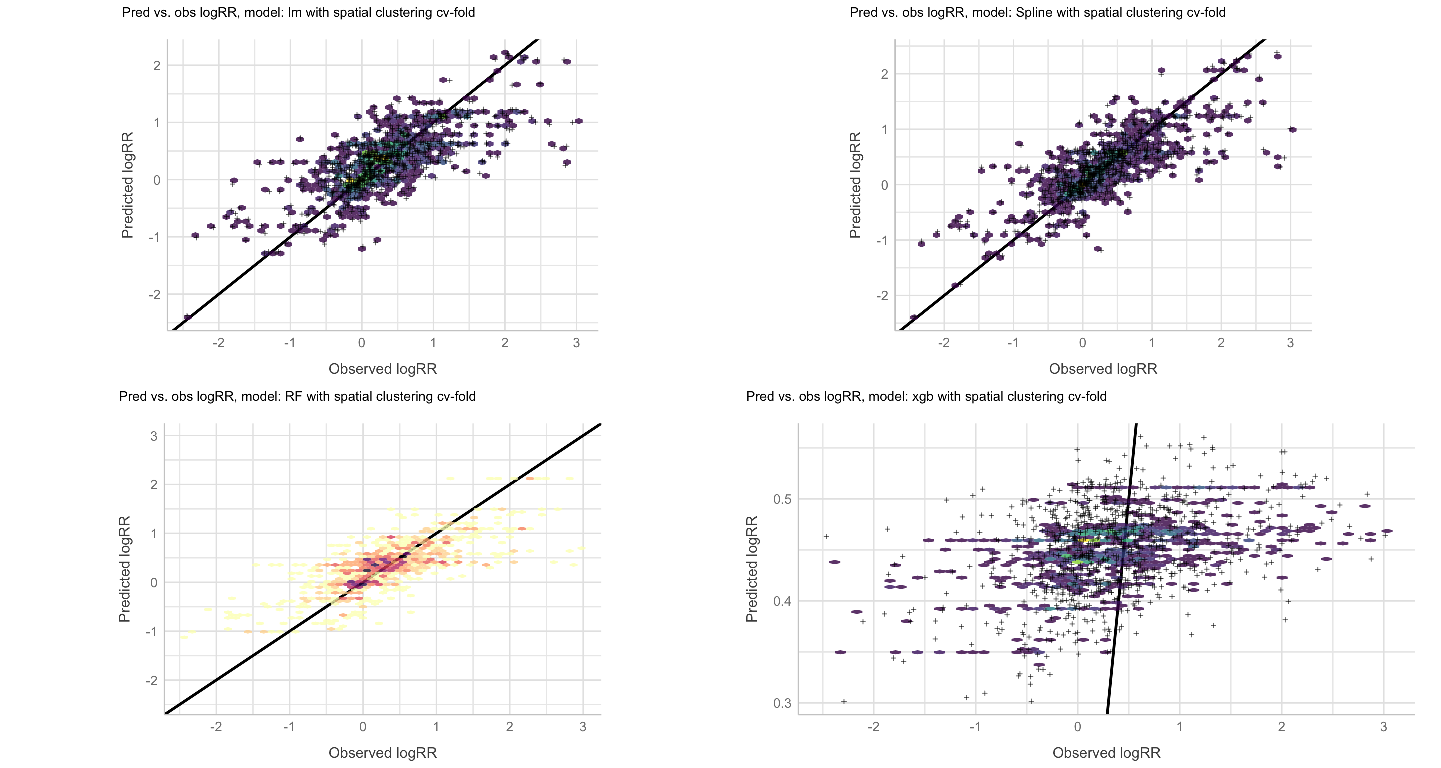
Figure 55: Predicted vs. observed logRR values, resampling: Spatial clustering cv-folds
Resampling: normal cv-folds
Show code
lm_cv_test_pred_hexplot <- readRDS(file = here::here("TidyMod_OUTPUT", "lm_cv_test_pred_hexplot.RDS"))
spline_cv_test_pred_hexplot <- readRDS(file = here::here("TidyMod_OUTPUT", "spline_cv_test_pred_hexplot.RDS"))
rf_cv_test_pred_hexplot <- readRDS(file = here::here("TidyMod_OUTPUT", "rf_cv_test_pred_hexplot.RDS"))
xgb_cv_test_pred_hexplot <- readRDS(file = here::here("TidyMod_OUTPUT", "xgb_cv_test_pred_hexplot.RDS"))
all_cv_pred_vs_obs_logRR_plot <-
gridExtra::grid.arrange(lm_cv_test_pred_hexplot + theme(legend.position="none"),
spline_cv_test_pred_hexplot + theme(legend.position="none"),
rf_cv_test_pred_hexplot + theme(legend.position="none"),
xgb_cv_test_pred_hexplot + theme(legend.position="none"),
ncol = 2,
nrow = 2)
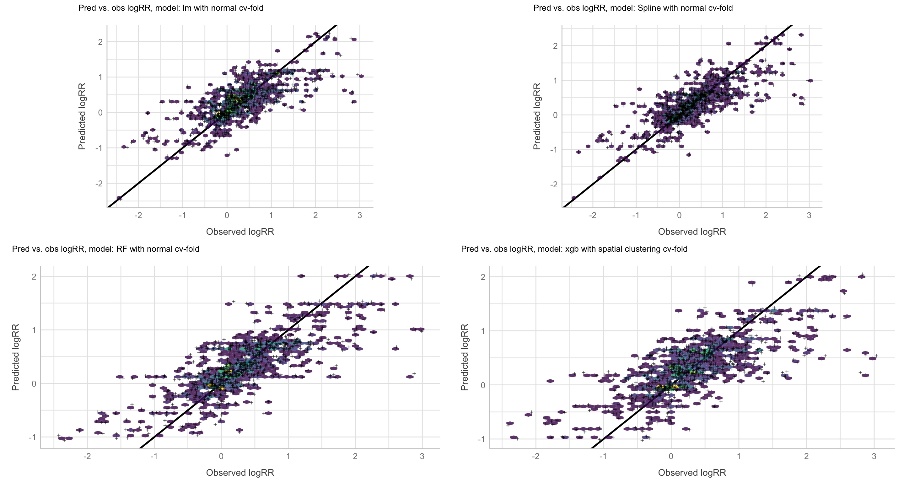
Figure 56: Predicted vs. observed logRR values, resampling: Normal cv-folds
STEP 11: Ensemble stacked modelling
Ensemble model, resampling: Spatial clustering cv-folds
The blend_predictions function determines how member model output will ultimately be combined in the final prediction, and is how we’ll calculate our stacking coefficients. Now that we know how to combine our model output, we can fit the models that we now know we need on the full training set. Any candidate ensemble member that has a stacking coefficient of zero doesn’t need to be refitted!
stacked_model_spatcv <- stacks::stacks() %>%
add_candidates(lm_fit_spatcv) %>%
add_candidates(glm_fit_spatcv) %>%
add_candidates(spline_fit_spatcv) %>%
add_candidates(knn_fit_spatcv) %>%
add_candidates(pca_fit_spatcv) %>%
add_candidates(rf_param_fit_spatcv) %>%
add_candidates(xgboost_param_fit_spatcv) %>%
add_candidates(catboost_param_fit_spatcv) %>%
add_candidates(lightgmb_param_fit_spatcv) %>%
blend_predictions(non_negative = TRUE,
penalty = 10^(-3:1),
mixture = 0.3,
metric = multi.metric) %>% # evaluate candidate models
fit_members() # fit non zero stacking coefficients
# Saving the stacked model ------------------ ------------------ ------------------ ------------------ ------------------
saveRDS(stacked_model_spatcv, file = here::here("TidyMod_OUTPUT", "stacked_model_spatcv.RDS"))
# ── A stacked ensemble model ─────────────────────────────────────
#
# Out of 90 possible candidate members, the ensemble retained 2.
# Penalty: 0.01.
# Mixture: 0.3.
#
# The 2 highest weighted members are:
Now that we’ve fitted the needed ensemble members, our model stack is ready to go! For the most part, a model stack is just a list that contains a bunch of ensemble members and instructions on how to combine their predictions.
Show code
# A tibble: 2 × 3
member type weight
<chr> <chr> <dbl>
1 lightgmb_param_fit_spatcv_1_14 boost_tree 0.624
2 xgboost_param_fit_spatcv_1_16 boost_tree 0.0190Stacking coeffecients
These stacking coefficients determine which candidate ensemble members will become ensemble members. Candidates with non-zero stacking coefficients are then fitted on the whole training set, altogether making up a model_stack object. We see that our model have choosen only two model candidates (LightGMB and XGBoost) out of 90 possible model candidates - and both of these two are tree-based models. 90 because each model has various unique (hyper)-parameter settings/combinations, resulting in several more candidates than actual model algorithms.
Show code
stacks::autoplot(stacked_model_spatcv, type = "weights") +
see::theme_lucid() +
ggtitle("Predicted vs. observed for stacked model fit using spatial clustering cv-folds") +
theme_lucid(plot.title.size = 25)
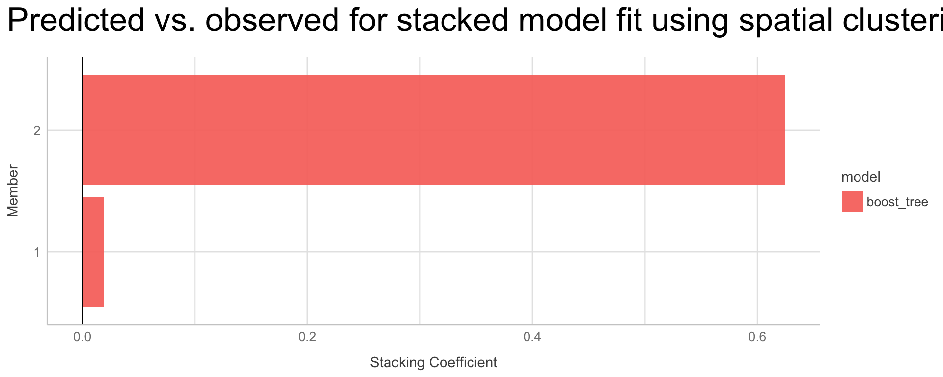
Figure 57: Stacking coeffecients, resampling: Spatial clustering cv-folds
Relation/trade-off between performance and the number of member candidates
To make sure that we have the right trade-off between minimizing the number of members and optimizing performance of the stacked model, we can use the stacks::autoplot() function. Below we see that the most optimal amount of members is also related to the LASSO penalty we give the stacking method as an argument.
Show code
stacks::autoplot(stacked_model_spatcv)
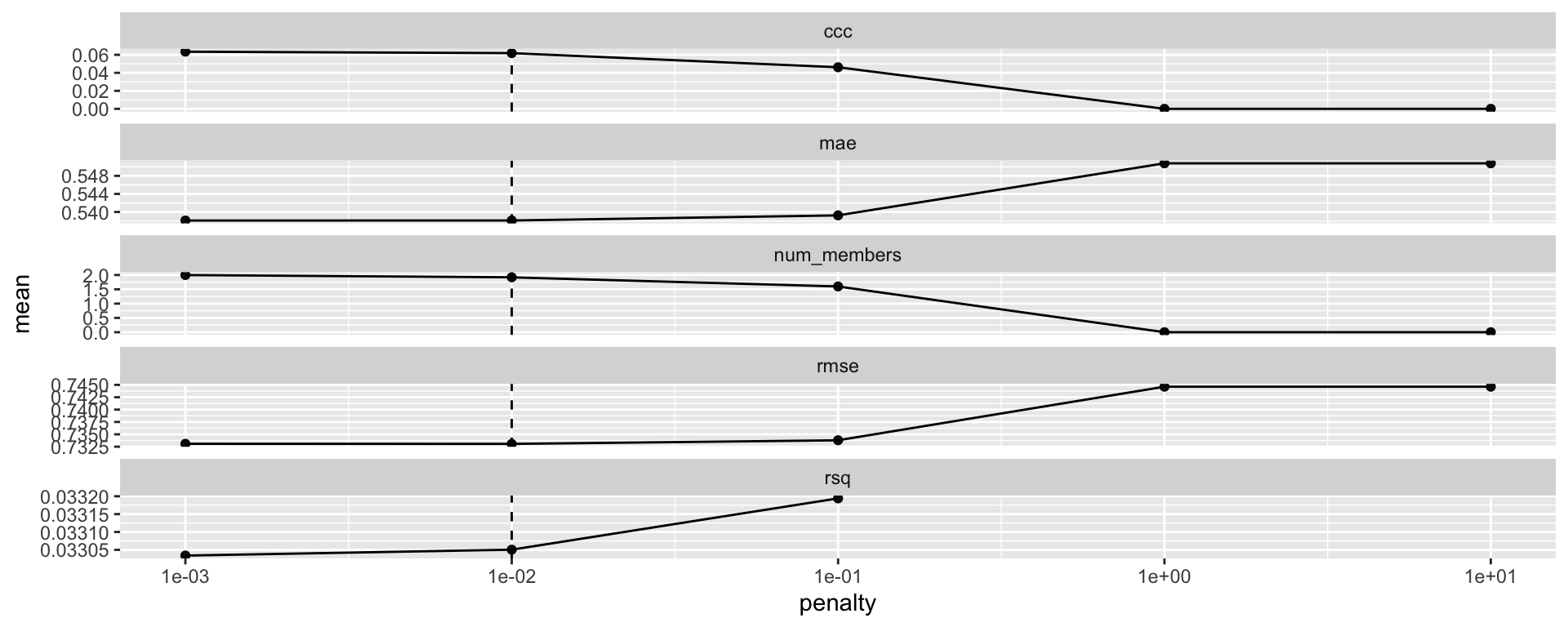
Figure 58: Trade-off between performance and the number of member candidates, resampling: Spatial clustering cv-folds
We can visualize this more clearly using the stacks::autoplot() argument, type and choose “members.”
Show code
stacks::autoplot(stacked_model_spatcv, type = "members") +
geom_line()
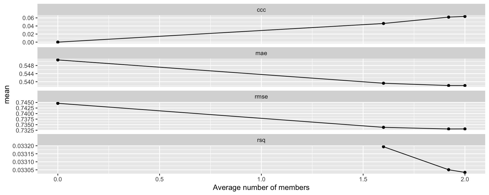
Figure 59: Number of member candidates, resampling: Spatial clustering cv-folds
With our two members we have indeed accomplished the best performance.
Visualising predicted vs. observed for the stacked model
Let us now finally visualise the relationship between predicted and observed logRR values for the ensemble stacked model when we use the stacked model to predict on our testing set.
# Pulling the testing set of the initial data splitting
test_data <- testing(af.split)
# Getting the predictions on the testing data using the Ensemble Stacked model
mod_pred_spatcv <- predict(stacked_model_spatcv, test_data) %>%
bind_cols(test_data)
stacked_pred_vs_obs_spatcv <-
ggplot(mod_pred_spatcv, aes(x = logRR, y = .pred)) +
#geom_point(alpha = 0.2) +
coord_obs_pred() +
labs(x = "Observed logRR", y = "Predicted logRR") +
#geom_abline(linetype = "dashed", col = "red", lty = 1, size = 1) +
geom_smooth(method = "gam", linetype = "dashed", col = "black", lty = 1, size = 1) +
geom_jitter(width = 0.2, height = 0.2, size = 0.2, shape = 10) +
coord_fixed(ratio = 0.8) +
geom_hex(bins = 50, alpha = 1, show.legend = FALSE) +
scale_fill_continuous(type = "viridis") +
ggtitle("Predicted vs. observed for stacked model fit using spatial clustering cv-folds") +
theme_lucid(plot.title.size = 25)
# Saving the stacked plot ------------------ ------------------ ------------------ ------------------ ------------------
saveRDS(stacked_pred_vs_obs_spatcv, file = here::here("TidyMod_OUTPUT", "stacked_pred_vs_obs_spatcv.RDS"))
Show code
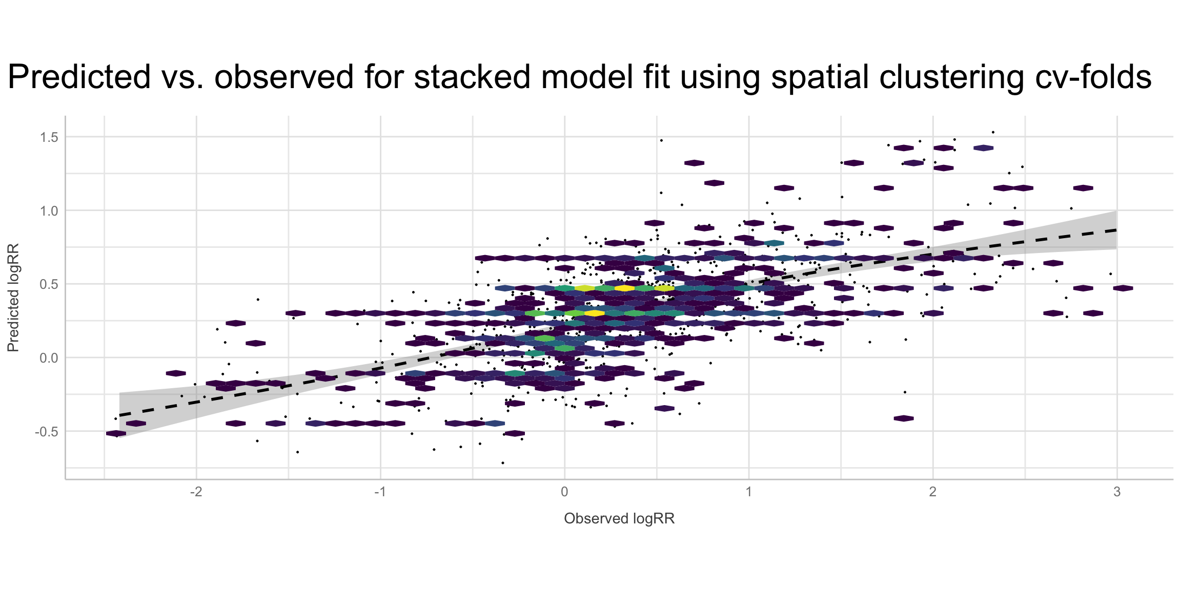
Figure 60: Predicted vs. observed for the stacked model, resampling: Spatial clustering cv-folds
Another simpler way of doing this could be using ggplot:
Show code
agrofor_test_spatcv <-
af.test %>%
bind_cols(predict(stacked_model_spatcv, .))
pred_vs_obs_simple_spatcv <-
ggplot(agrofor_test_spatcv) +
aes(x = logRR,
y = .pred) +
geom_point() +
coord_obs_pred()
# Saving the stacked plot ------------------ ------------------ ------------------ ------------------ ------------------
saveRDS(pred_vs_obs_simple_spatcv, file = here::here("TidyMod_OUTPUT", "pred_vs_obs_simple_spatcv.RDS"))
Show code
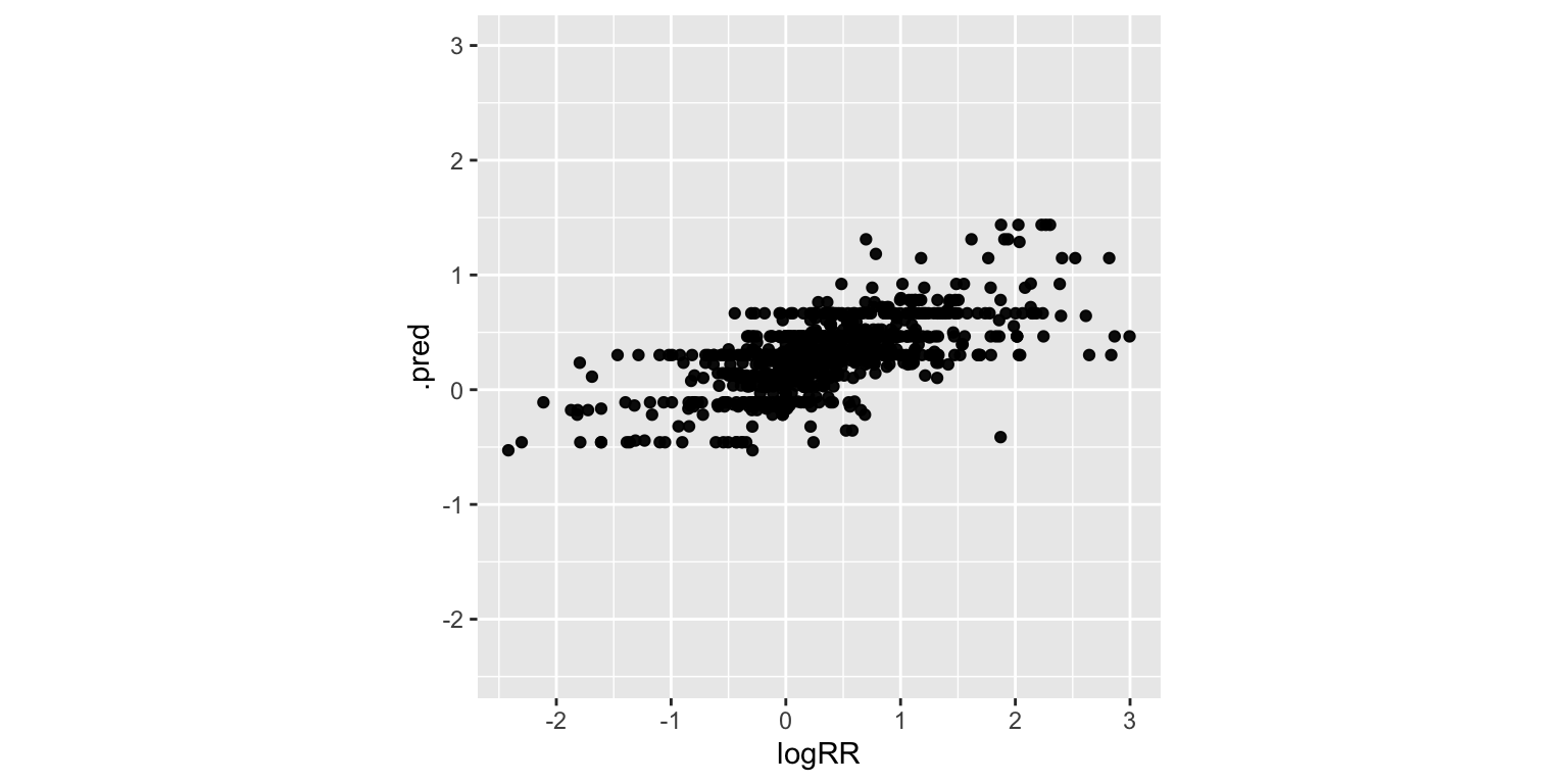
Figure 61: Simple plot for pred vs. obs for the stacked model, resampling: Spatial clustering cv-folds
Looks like our predictions were pretty strong! How do the stacks predictions perform, though, as compared to the members’ predictions? We can use the type = “members” argument to generate predictions from each of the ensemble members.
Lares regression performance plot, ensemble stacked model fit with spatial clustering cv-folds
The lares package is an R package built to automate, improve, and speed everyday analysis and machine learning tasks, build specifically for visualising regression and classification model performance by easily and intuitively giving most important plots, all generated at once. Lets see how our stacked model performs using the lares package function mplot_full(). This function plots a whole dashboard with a model’s results. It will automatically detect if it’s a categorical or regression’s model by checking how many different unique values the independent variable (tag) has. This will give us multiple plots gathered into one, showing tag vs score performance results.
Show code
agfor_stacked_model_full_lares_plot_spatcv <-
lares::mplot_full(tag = mod_pred_spatcv$logRR,
score = mod_pred_spatcv$.pred,
splits = 10,
subtitle = "Results of Regression of Ensemble Stacked Model on models fit with spatial clustering cv-folds",
model_name = "Ensemble Stacked Model with models fit using spatial clustering cv-folds",
save = TRUE,
file_name = "agfor_stacked_model_full_lares_plot_spatcv.png",
plot = FALSE)
Show code
ggdraw() +
draw_image(here::here("TidyMod_OUTPUT", "agfor_stacked_model_full_lares_plot_spatcv.png"))
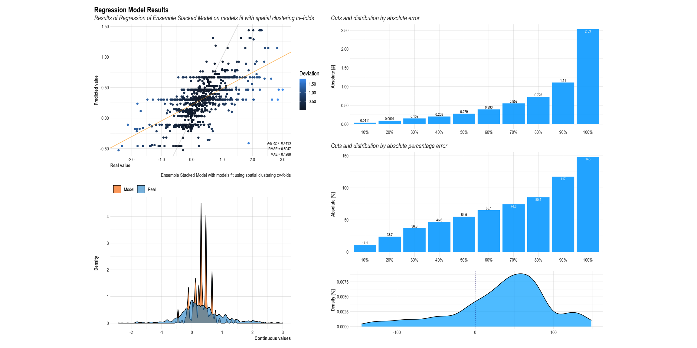
Figure 62: Full lares plot for the ensemble stacked model with spatial clustering cv-folds
Show code
agfor_stacked_model_linear_lares_plot_spatcv <-
lares::mplot_lineal(tag = mod_pred_spatcv$logRR,
score = mod_pred_spatcv$.pred,
subtitle = "Regression of Ensemble Stacked Model, resampling: spatial clustering cv-folds",
model_name = "Regression of Ensemble Stacked Model with only linear",
save = TRUE,
file_name = "agfor_stacked_model_linreg_lares_plot_spatcv.png")
Show code
ggdraw() +
draw_image(here::here("TidyMod_OUTPUT", "agfor_stacked_model_linreg_lares_plot_spatcv.png"))
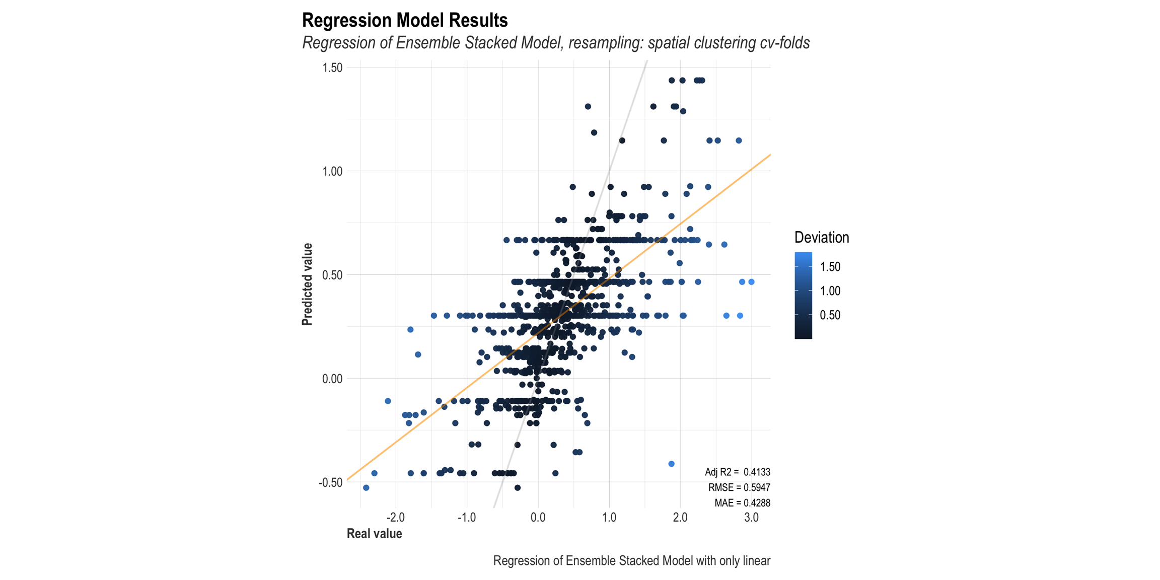
Figure 63: Lares linear regression plot for the ensemble stacked model with spatial clustering cv-folds
Model performance in splits by quantiles
One of my favourite functions to study our model’s quality is the following. What it shows is the result of arranging all scores or predicted values in sorted quantiles, from worst to best, and see how the classification goes compared to our test set. The math behind this plot might be a bit foggy so lets try to explain further: if we sort all our observations from the lowest to the highest, then we can, for instance, select the top 5 or bottom 15 % or so. What we do now is split all those “ranked” rows into similar-sized-buckets to get the best bucket, the second-best one, and so on. Then, if we split all the “goods” and the “bads” into five columns, keeping their buckets’ colours, we still have it sorted and separated, right?
agfor_stacked_model_splits_lares_plot_spatcv <-
lares::mplot_splits(tag = mod_pred_spatcv$logRR,
score = mod_pred_spatcv$.pred,
split = 5,
save = TRUE,
file_name = "agfor_stacked_model_splits_lares_plot_spatcv.png",
subtitle = "Lares split by group plot for stacked ensemble model, resampling: Spatial clustering cv-folds")
Show code
ggdraw() +
draw_image(here::here("TidyMod_OUTPUT", "agfor_stacked_model_splits_lares_plot_spatcv.png"))
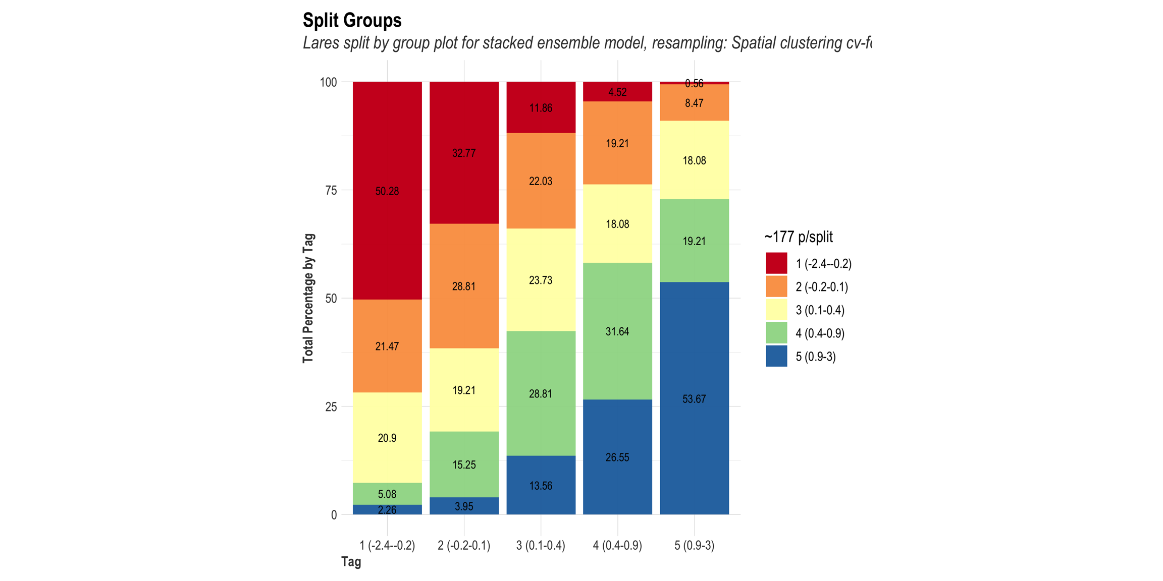
Figure 64: Lares linear regression plot for the ensemble stacked model with normal cv-folds
Comparing RMSE (or any other metric) of individual models with the ensemble stacked model
Now, let us evaluate the root mean squared error from each model compared to the ensemble stacked model
member_preds_spatcv <-
af.test %>%
select(logRR) %>%
bind_cols(predict(stacked_model_spatcv, af.test, members = TRUE))
member_map_preds_spatcv <-
map_dfr(member_preds_spatcv, rmse, truth = logRR, data = member_preds_spatcv) %>%
mutate(member = colnames(member_preds_spatcv))
# Saving the stacked data for member_map_preds_spatcv ------------------ ------------------ ------------------ ------------------ ------------------
saveRDS(member_map_preds_spatcv, file = here::here("TidyMod_OUTPUT", "member_map_preds_spatcv.RDS"))
Show code
member_map_preds_spatcv <- readRDS(file = here::here("TidyMod_OUTPUT", "member_map_preds_spatcv.RDS"))
rmarkdown::paged_table(member_map_preds_spatcv)
Ensemble model, resampling: Normal cv-folds
Show code
stacked_model_cv <- stacks::stacks() %>%
add_candidates(lm_fit_cv) %>%
add_candidates(glm_fit_cv) %>%
add_candidates(spline_fit_cv) %>%
add_candidates(knn_fit_cv) %>%
add_candidates(pca_fit_cv) %>%
add_candidates(rf_param_fit_cv) %>%
add_candidates(xgboost_param_fit_cv) %>%
add_candidates(catboost_param_fit_cv) %>%
add_candidates(lightgmb_param_fit_cv) %>%
blend_predictions(non_negative = TRUE,
penalty = 10^(-3:1),
mixture = 1,
metric = multi.metric) %>% # evaluate candidate models
fit_members() # fit non zero stacking coefficients
# Saving the stacked model ------------------ ------------------ ------------------ ------------------ ------------------
saveRDS(stacked_model_cv, file = here::here("TidyMod_OUTPUT", "stacked_model_cv.RDS"))
# ── A stacked ensemble model ─────────────────────────────────────
#
# Out of 90 possible candidate members, the ensemble retained 9.
# Penalty: 0.01.
# Mixture: 1.
#
# The 9 highest weighted members are:
Show code
# A tibble: 9 × 3
member type weight
<chr> <chr> <dbl>
1 xgboost_param_fit_cv_1_20 boost_tree 3234.
2 xgboost_param_fit_cv_1_17 boost_tree 6.60
3 rf_param_fit_cv_1_03 rand_forest 0.259
4 xgboost_param_fit_cv_1_16 boost_tree 0.220
5 xgboost_param_fit_cv_1_15 boost_tree 0.126
6 rf_param_fit_cv_1_19 rand_forest 0.121
7 lightgmb_param_fit_cv_1_15 boost_tree 0.0981
8 spline_fit_cv_1_1 linear_reg 0.00777
9 rf_param_fit_cv_1_10 rand_forest 0.0000798Show code
stacks::autoplot(stacked_model_cv)

Figure 65: Stacking coeffecients, resampling: Normal cv-folds
Show code
stacks::autoplot(stacked_model_cv, type = "members") +
geom_line()
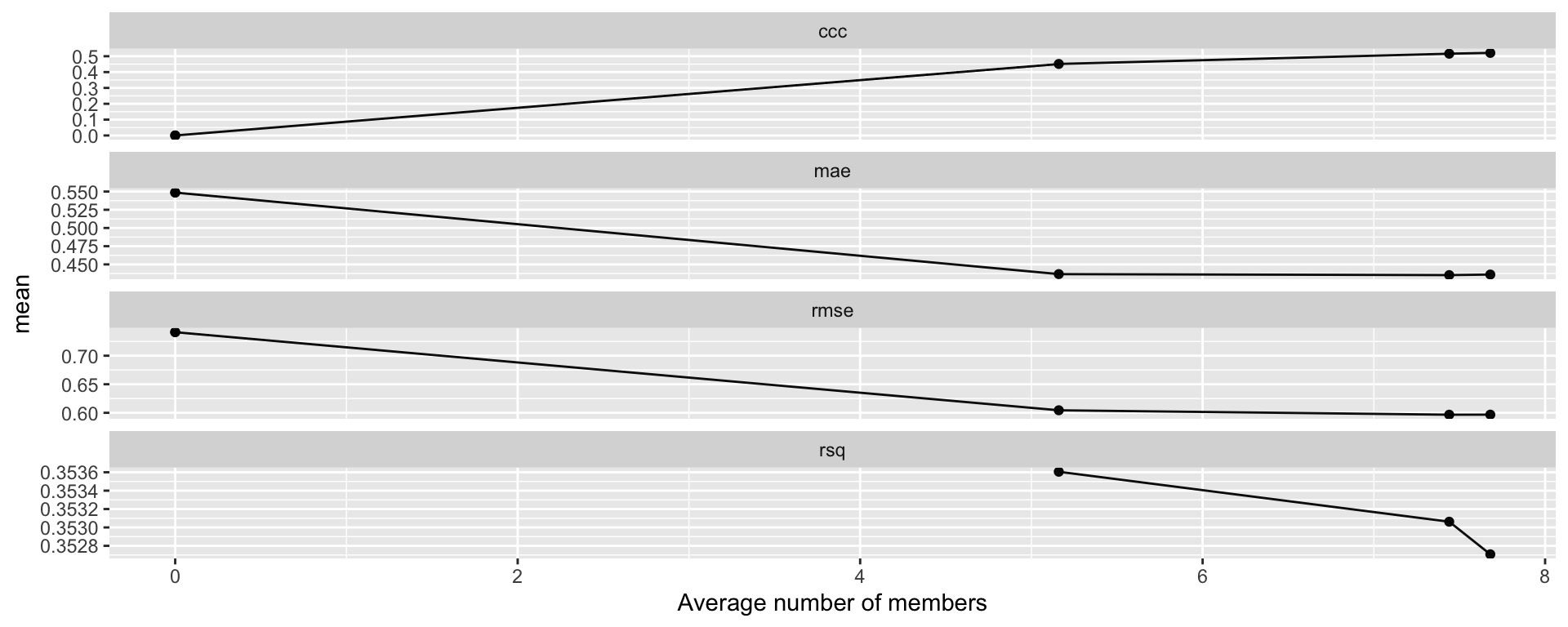
Figure 66: Trade-off between performance and the number of member candidates, resampling: Normal cv-folds
We can visualize this more clearly using the stacks::autoplot() argument, type and choose “members.”
Show code
stacks::autoplot(stacked_model_cv, type = "weights") +
scale_x_continuous(trans = 'log2') +
see::theme_lucid()
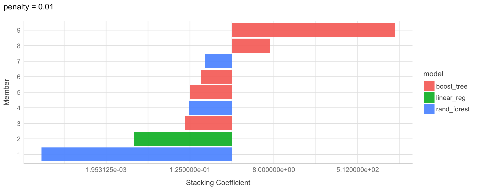
Figure 67: Number of member candidates, resampling: Normal cv-folds
We see that there are some members (model candidates) that have been included even though they are negatively contributing to the stacks. There can be several logical reasons for this.
Visualising predicted vs. observed for the stacked model
# Pulling the testing set of the initial data splitting
test_data <- testing(af.split)
# Getting the predictions on the testing data using the Ensemble Stacked model
mod_pred_cv <- predict(stacked_model_cv, test_data) %>%
bind_cols(test_data)
stacked_pred_vs_obs_cv <-
ggplot(mod_pred_cv, aes(x = logRR, y = .pred)) +
#geom_point(alpha = 0.2) +
coord_obs_pred() +
labs(x = "Observed logRR", y = "Predicted logRR") +
geom_abline(linetype = "dashed", col = "red", lty = 1, size = 1) +
#geom_smooth(method = "gam", linetype = "dashed", col = "black", lty = 1, size = 1) +
geom_jitter(width = 0.2, height = 0.2, size = 0.2, shape = 10) +
coord_fixed(ratio = 0.8) +
geom_hex(bins = 50, alpha = 1, show.legend = FALSE) +
scale_fill_continuous(type = "viridis") +
ggtitle("Predicted vs. observed for stacked model fit using normal cv-folds") +
theme_lucid(plot.title.size = 25)
# Saving the stacked plot ------------------ ------------------ ------------------ ------------------ ------------------
saveRDS(stacked_pred_vs_obs_cv, file = here::here("TidyMod_OUTPUT", "stacked_pred_vs_obs_cv.RDS"))
Show code
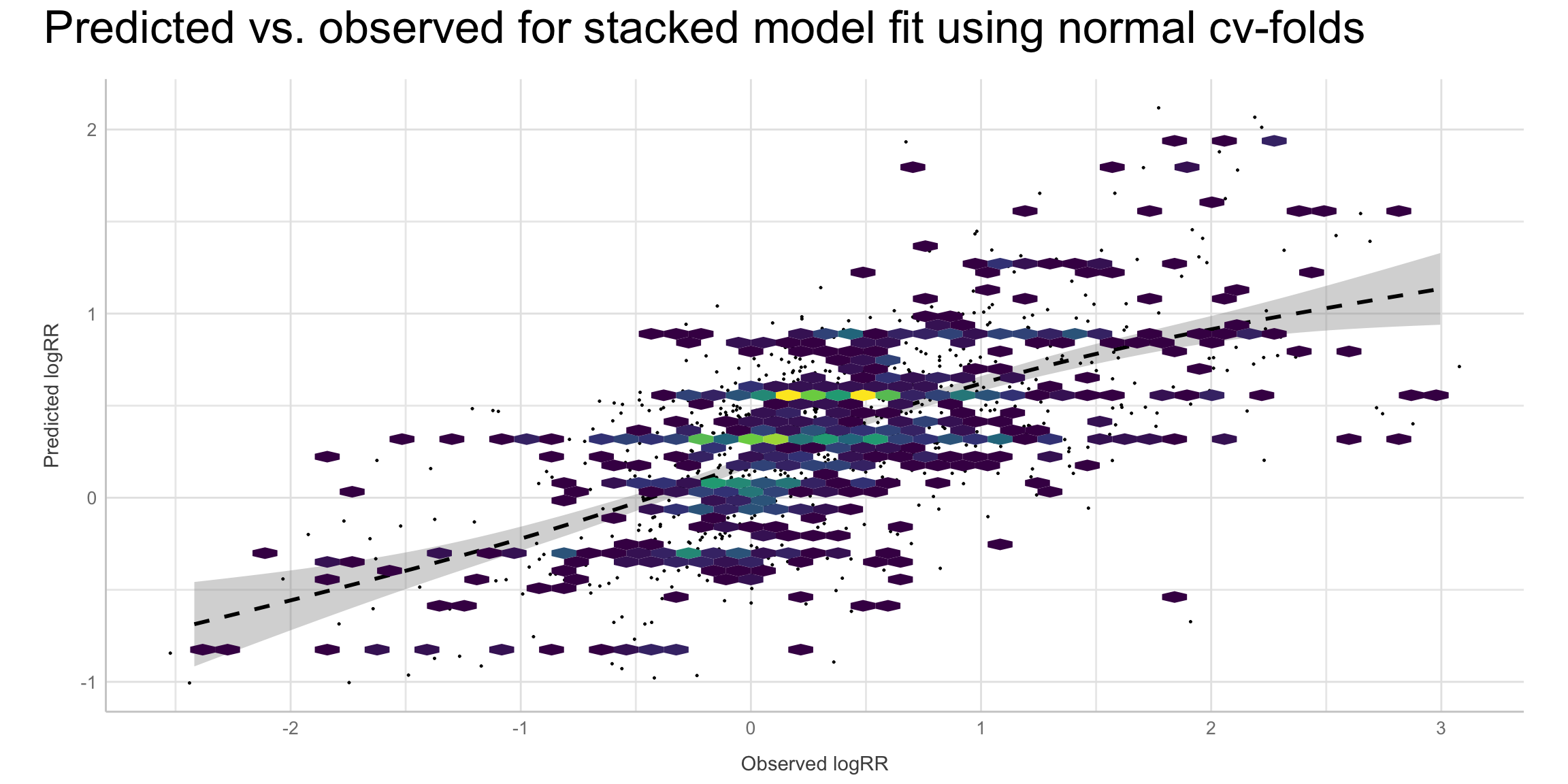
Figure 68: Predicted vs. observed for the stacked model, resampling: Normal cv-folds
Another simpler way of doing this could be using ggplot:
Show code
agrofor_test_cv <-
af.test %>%
bind_cols(predict(stacked_model_cv, .))
pred_vs_obs_simple_cv <-
ggplot(agrofor_test_cv) +
aes(x = logRR,
y = .pred) +
geom_point() +
coord_obs_pred()
# Saving the stacked plot ------------------ ------------------ ------------------ ------------------ ------------------
saveRDS(pred_vs_obs_simple_cv, file = here::here("TidyMod_OUTPUT", "pred_vs_obs_simple_cv.RDS"))
Show code

Figure 69: Simple plot for pred vs. obs for the stacked model, resampling: Normal cv-folds
Lares regression performance plot, ensemble stacked model fit with normal cv-folds
agfor_stacked_model_full_lares_plot_cv <-
lares::mplot_full(tag = mod_pred_cv$logRR,
score = mod_pred_cv$.pred,
splits = 10,
subtitle = "Results of Regression of Ensemble Stacked Model on models fit with normal cv-folds",
model_name = "Ensemble Stacked Model with models fit using normal cv-folds",
save = TRUE,
file_name = "agfor_stacked_model_full_lares_plot_cv.png",
plot = FALSE)
Show code
ggdraw() +
draw_image(here::here("TidyMod_OUTPUT","agfor_stacked_model_full_lares_plot_cv.png"))

Figure 70: Full lares plot for the ensemble stacked model with normal cv-folds
Show code
agfor_stacked_model_linear_lares_plot_cv <-
lares::mplot_lineal(tag = mod_pred_cv$logRR,
score = mod_pred_cv$.pred,
subtitle = "Regression of Ensemble Stacked Model, resampling: Normal cv-folds",
model_name = "Regression of Ensemble Stacked Model with only linear",
save = TRUE,
file_name = "agfor_stacked_model_linreg_lares_plot_cv.png")
Show code
ggdraw() +
draw_image(here::here("TidyMod_OUTPUT", "agfor_stacked_model_linreg_lares_plot_cv.png"))
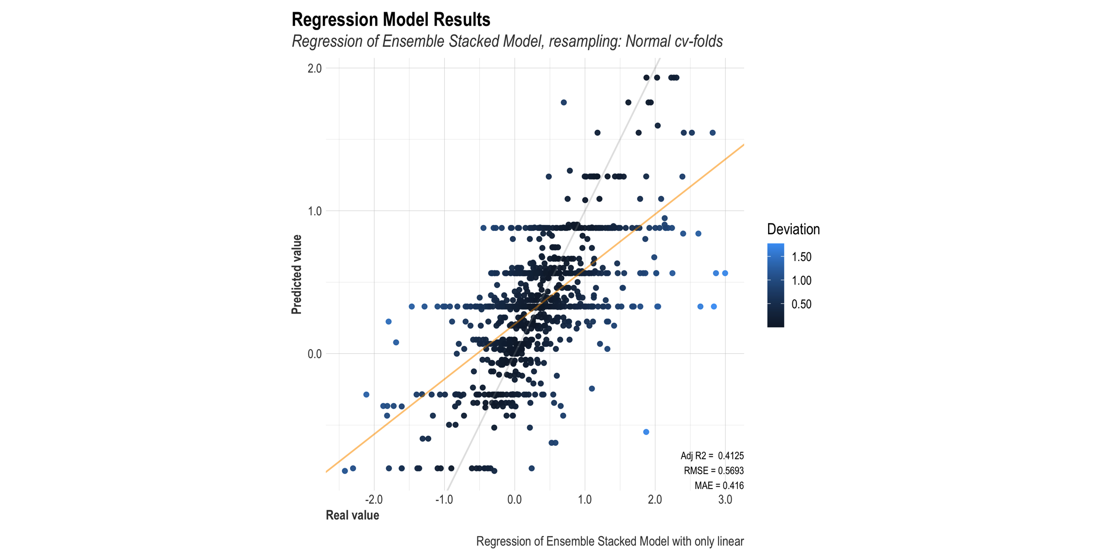
Figure 71: Full lares plot for the ensemble stacked model with normal cv-folds
Lares splits for the models fit with normal cv-folds
agfor_stacked_model_split_lares_plot_cv <-
lares::mplot_splits(tag = mod_pred_cv$logRR,
score = mod_pred_cv$.pred,
split = 5,
save = TRUE,
file_name = "agfor_stacked_model_splits_lares_plot_cv.png",
subtitle = "Lares split by group plot for stacked ensemble model, resampling: Normal cv-folds")
Show code
ggdraw() +
draw_image(here::here("TidyMod_OUTPUT","agfor_stacked_model_splits_lares_plot_cv.png"))
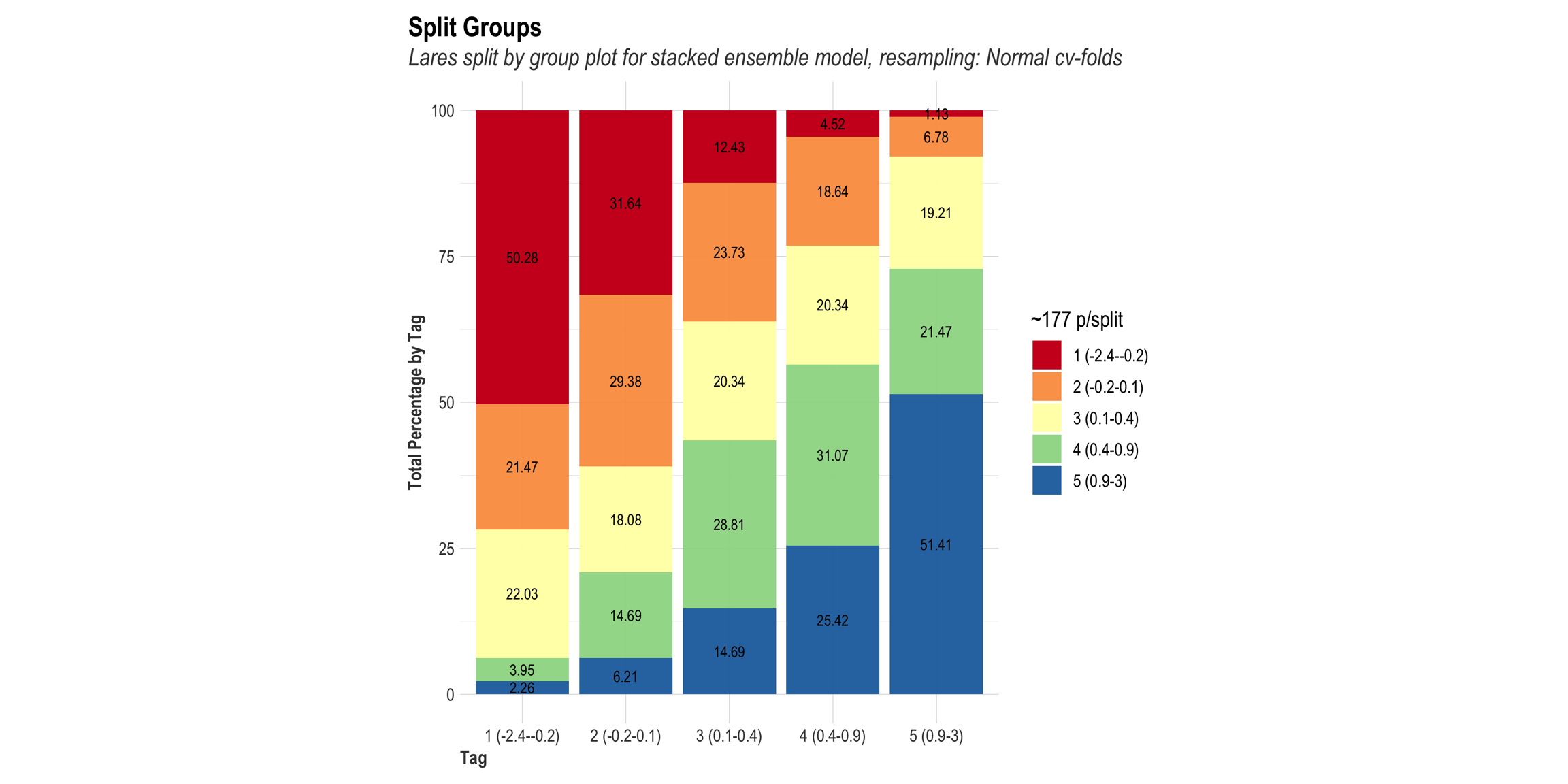
Figure 72: Splits lares plot for the ensemble stacked model with normal cv-folds
Comparing RMSE (or any other metric) of individual models with the ensemble stacked model
Now, let us evaluate the root mean squared error from each model compared to the ensemble stacked model
member_preds_cv <-
af.test %>%
select(logRR) %>%
bind_cols(predict(stacked_model_cv, af.test, members = TRUE))
member_map_preds_cv <-
map_dfr(member_preds_cv, rmse, truth = logRR, data = member_preds_cv) %>%
mutate(member = colnames(member_preds_cv))
# Saving the stacked data for member_map_preds_spatcv ------------------ ------------------ ------------------ ------------------ ------------------
saveRDS(member_map_preds_cv, file = here::here("TidyMod_OUTPUT", "member_map_preds_cv.RDS"))
Show code
member_map_preds_cv <- readRDS(file = here::here("TidyMod_OUTPUT", "member_map_preds_cv.RDS"))
rmarkdown::paged_table(member_map_preds_cv)
As we can see, the stacked ensemble outperforms each of the member models, though is closely followed by one of its members.
Voila! We’ve now made use of the stacks package to predict response ratioe outcomes of ERA agroforestry data observations from ERA using a stacked ensemble modelling approach!
Amazon Elastic Compute Cloud is a part of Amazon.com’s cloud-computing platform, Amazon Web Services (AWS), that allows users to rent virtual computers on which to run their own computer applications.↩︎