Loading necessary R packages and ERA data
Loading general R packages
This part of the document is where we actually get to the nitty-gritty of the ERA agroforestry data and therefore it requires us to load a number of R packages for both general Explorortive Data Analysis and Machine Learning.
Show code
# Using the pacman functions to load required packages

        if(!require("pacman", character.only = TRUE)){
          install.packages("pacman",dependencies = T)
          }

# ------------------------------------------------------------------------------------------
# General packages
# ------------------------------------------------------------------------------------------
required.packages <- c("tidyverse", "tidymodels", "finetune", "kernlab", "here", "hablar", "spatialsample", "GGally", "klaR", "cowplot",
                       "stacks", "rules", "baguette", "viridis", "yardstick", "DALEXtra", "discrim", "themis", "corrr",
# ------------------------------------------------------------------------------------------
# Parallel computing packages
# ------------------------------------------------------------------------------------------
                      "parallelMap", "parallelly", "parallel", "doParallel"
)

p_load(char=required.packages, install = T,character.only = T)
STEP 1: Getting the data
Discritization of target feature, logRR i) Boxplots of predictors vs. discritized logRR
We are now going to discretize our continues outcome feature, logRR into seven categorical/nominal groups. In statistics and machine learning, discretization refers to the process of converting or partitioning continuous features into discretized or nominal features with certain intervals. The goal of discretization is to reduce the number of values a continuous feature have by grouping it into a number of intervals or bins. This can be useful when one wish to perform EDA on a continues feature with no or very little linear (co)-relation to predictors. Hence, we can group the continuous outcome feature, logRR and look at discrete differences on the predictors for each group of logRR. Continuous features have a smaller chance of correlating with the target variable due to infinite degrees of freedom and may have a complex non-linear relationship. After discretizing logRR into groups it it easier to perform test on differences and for these results to be interpreted. The aim of performing the discretization of logRR in our case is to be able to make a pairwise t-test for the different groups of logRR. Thereby getting an understanding of whether there is significant differences between levels of logRR. Discretization, or binning/grouping of a continuous feature is mostly done in two ways, and we are going to evaluate the t-test outcome from both of these methods - because the binning technique is so different:
Equal-Width Discretization: Separating all possible values into ‘N’ number of bins, each having the same width. Formula for interval width: Width = (maximum value - minimum value) / N. Where N is the number of bins or intervals. This method doesn’t improve the value spread and it can handle outliers effectively.
Equal-Frequency Discretization: Separating all possible values into ‘N’ number of bins, each having the same amount of observations. These intervals are normally corresponding to ranges or quantile values. This method does improve the value spread and it can handle outliers effectively.
First, we are creating a two new feature columns in our agroforestry modelling data. We are using the functions cut_interval() and cut_number(), to perform the discrete levels of logRR based on the equal-frequency method and the equal-width method, respectfully. For each method seven groups are created. The groups range from 1, extremely low (low logRR values) to 7, extremely high (high logRR values).
STEP 1: Performing EQNo and EQR discretization
agrofor.biophys.modelling.data.class <-  agrofor.biophys.modelling.data %>%
  dplyr::select(-c("RR", "ID", "AEZ16s", "Country", "MeanC", "MeanT", "PrName.Code", "SubPrName"))

agrofor.biophys.modelling.data.discretized.logRR <- agrofor.biophys.modelling.data.class %>%
  rationalize(logRR) %>%
  drop_na(logRR) %>%
  mutate(logRR_counts_cut_interval = cut_interval(logRR, n = 7)) %>%
  mutate(logRR_EQR_group = case_when(
    logRR_counts_cut_interval   == "[-4.43,-3.16]"   ~ "1.extremely_low",
    logRR_counts_cut_interval   == "(-3.16,-1.9]"    ~ "2.very_low",
    logRR_counts_cut_interval   == "(-1.9,-0.627]"   ~ "3.low",
    logRR_counts_cut_interval   == "(-0.627,0.642]"  ~ "4.medium",
    logRR_counts_cut_interval   == "(0.642,1.91]"    ~ "5.high",
    logRR_counts_cut_interval   == "(1.91,3.18]"     ~ "6.very_high",
    logRR_counts_cut_interval   == "(3.18,4.45]"     ~ "7.extremely_high",)) %>%

  mutate(logRR_counts_cut_number = cut_number(logRR, n = 7)) %>%
  mutate(logRR_EQNo_group = case_when(
    logRR_counts_cut_number   == "[-4.43,-0.31]"     ~ "1.extremly_low",
    logRR_counts_cut_number   == "(-0.31,-0.0195]"   ~ "2.very_low",
    logRR_counts_cut_number   == "(-0.0195,0.155]"   ~ "3.low",
    logRR_counts_cut_number   == "(0.155,0.379]"     ~ "4.medium",
    logRR_counts_cut_number   == "(0.379,0.643]"     ~ "5.high",
    logRR_counts_cut_number   == "(0.643,1.1]"       ~ "6.very_high",
    logRR_counts_cut_number   == "(1.1,4.45]"        ~ "7.extremely_high",))
Lets compare the newly created factor levels. Are there differences in how logRR was grouped by the two methods..?
Show code
rmarkdown::paged_table(agrofor.biophys.modelling.data.discretized.logRR %>%
  sample_n(25) %>% # randomly sampling a subset of 25 rows/observations
  dplyr::relocate(logRR_EQNo_group, logRR_EQR_group, logRR))
EQNo discretization
Show code
#Correlation Matrix Plot
ggparis.EQNo <-
  ggpairs(discretized.logRR.EQNo %>% dplyr::select(contains("SAND"),
                                          contains("iSDA_log_P"),
                                          contains("Bio01_MT_Annu"),
                                          contains("Bio17_Precip_DryQ"),
                                          contains("iSDA_log_C_tot"),
                                          contains("logRR_EQNo_group")),
        ggplot2::aes(color = logRR_EQNo_group, alpha = 0.3)) +
  theme_minimal() +
  scale_fill_viridis_d(aesthetics = c("color", "fill"), begin = 0.1, end = 0.8) +
  labs(title = "Numeric Bivariate Analysis of logRR_EQNo_group")
Show code
ggdraw() +
  draw_image(here::here("TidyMod_Class_OUTPUT", "NumBivAnalysis.EQNo.png"))
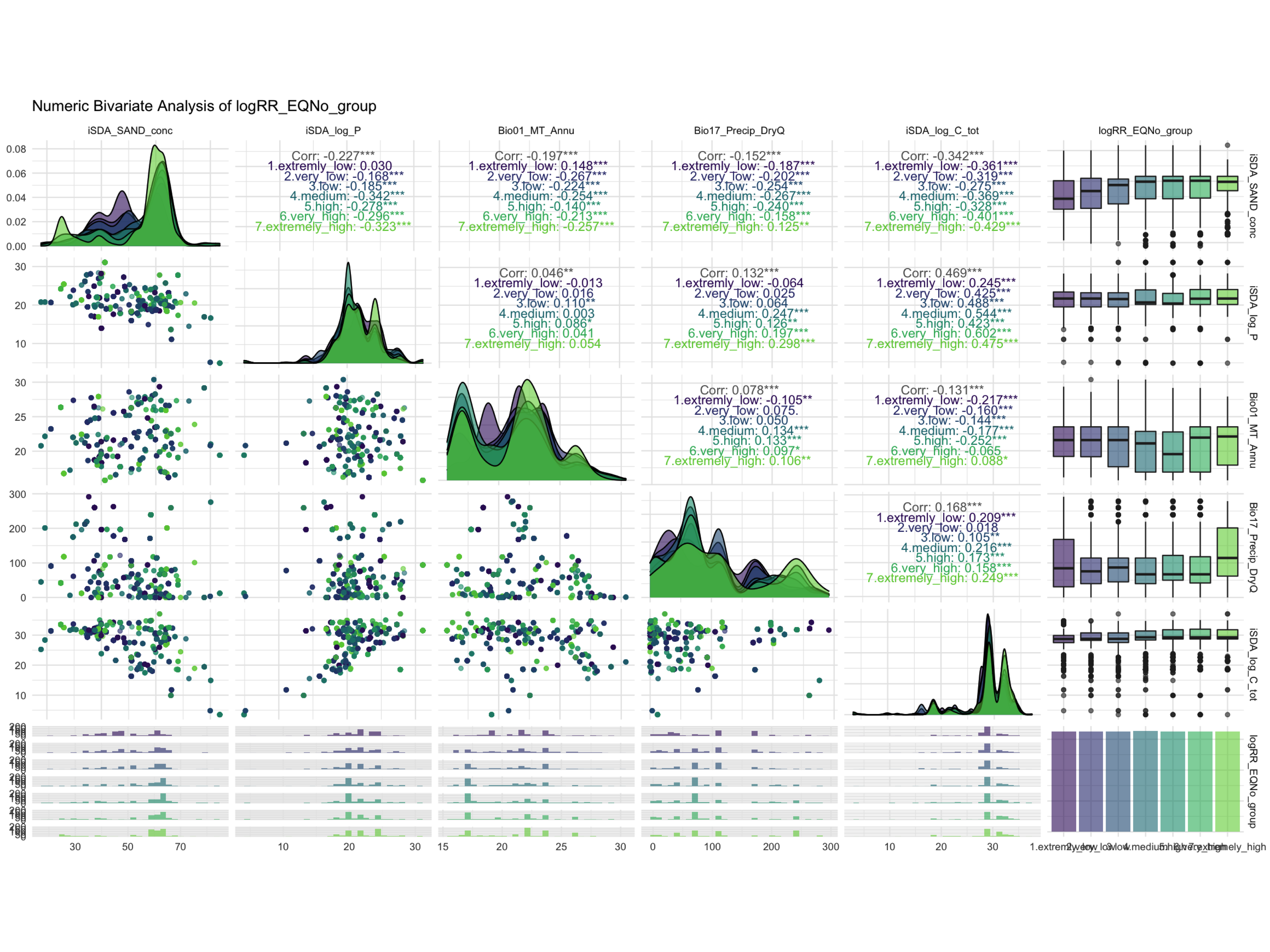
Figure 1: Numeric Bivariate Analysis of logRR_EQNo_group
EQR discretization
Show code
#Correlation Matrix Plot
ggparis.EQR <-
  ggpairs(discretized.logRR.EQR %>% dplyr::select(contains("SAND"),
                                          contains("iSDA_log_P"),
                                          contains("Bio01_MT_Annu"),
                                          contains("Bio17_Precip_DryQ"),
                                          contains("iSDA_log_C_tot"),
                                          contains("logRR_EQR_group")),
        ggplot2::aes(color = logRR_EQR_group, alpha = 0.3)) +
  theme_minimal() +
  scale_fill_viridis_d(aesthetics = c("color", "fill"), begin = 0.1, end = 0.8) +
  labs(title = "Numeric Bivariate Analysis of logRR_EQNo_group")
Show code
ggdraw() +
  draw_image(here::here("TidyMod_Class_OUTPUT", "NumBivAnalysis.EQR.png"))
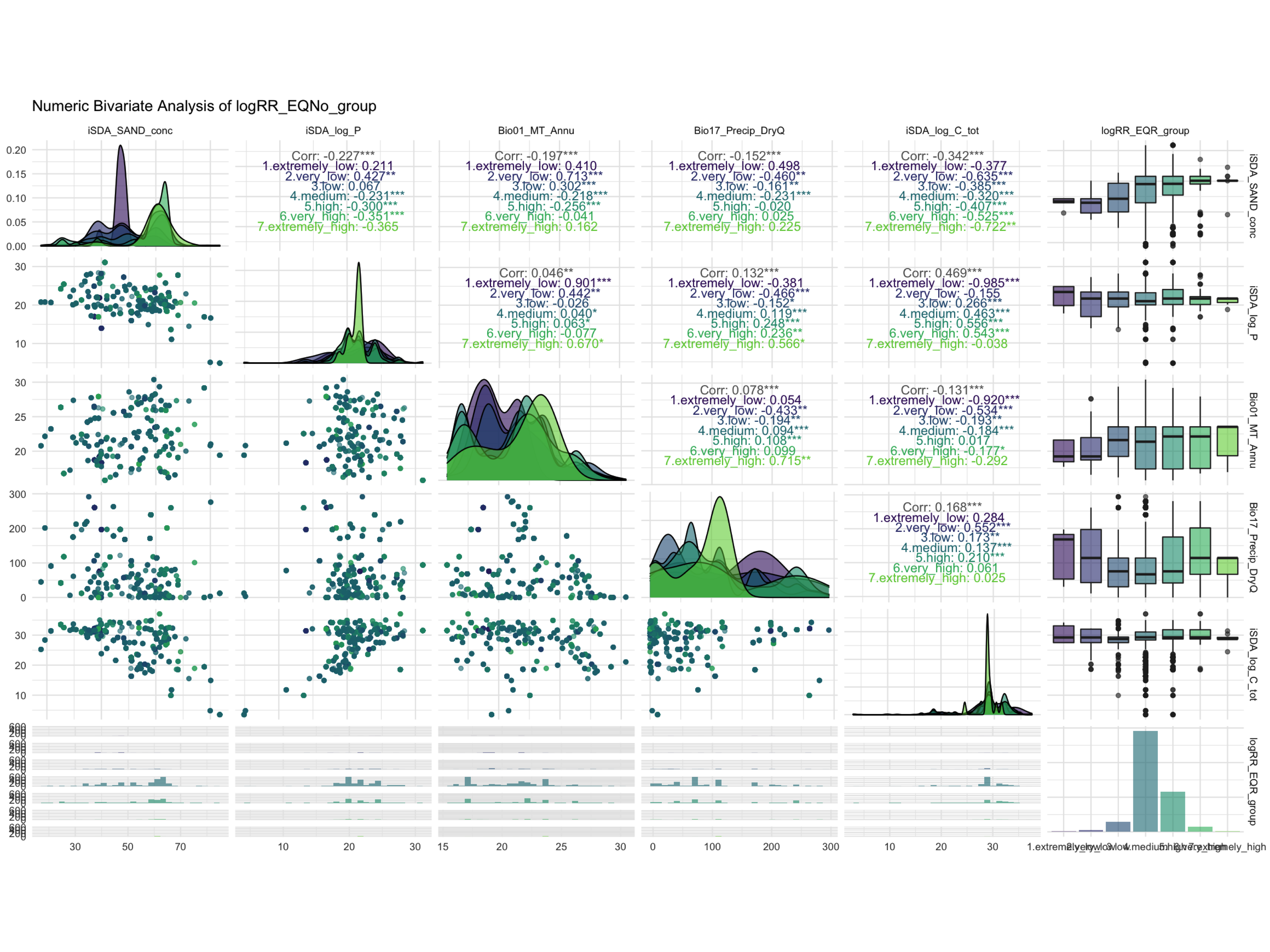
Figure 2: Numeric Bivariate Analysis of logRR_EQR_group
We now proceed with the dataset that has been discretized with the EQR method because this method seems to have the clearest separation of RR groups.
STEP 2: Splitting data
Split data in training and testing sets
set.seed(456)

# Splitting data
af.split.class <- initial_split(discretized.logRR.EQR, prop = 0.80, strata = logRR_EQR_group)

af.train.class <- training(af.split.class)
af.test.class <- testing(af.split.class)
STEP 3: Defining resampling techniques and global modelling metrics
# Re-sample technique(s)
cv_fold <- vfold_cv(af.train.class, v = 5)
STEP 4: Defining models
#Initialise Seven Models for Screening
nb_mod <-
  naive_Bayes(smoothness = tune(), Laplace = tune()) %>%
  set_engine("klaR") %>%
  set_mode("classification")

logistic_mod <-
  logistic_reg(penalty = tune(), mixture = tune()) %>%
  set_engine("glmnet") %>%
  set_mode("classification")

dt_mod <- decision_tree(cost_complexity = tune(), tree_depth = tune(), min_n = tune()) %>%
  set_engine("rpart") %>%
  set_mode("classification")

rf_mod <-
  rand_forest(mtry = tune(), trees = tune(), min_n = tune()) %>%
  set_engine("ranger") %>%
  set_mode("classification")

knn_mod <- nearest_neighbor(neighbors = tune(), weight_func = tune(), dist_power = tune()) %>%
  set_engine("kknn") %>%
  set_mode("classification")

svm_mod <-
  svm_rbf(cost = tune(), rbf_sigma = tune(), margin = tune()) %>%
  set_engine("kernlab") %>%
  set_mode("classification")

xgboost_mod <- boost_tree(mtry = tune(), trees = tune(), min_n = tune(), tree_depth = tune(), learn_rate = tune(), loss_reduction = tune(), sample_size = tune())  %>%
  set_engine("xgboost") %>%
  set_mode("classification")
STEP 5: Create pre-processing recipies
base_recipe <-
  recipe(formula = logRR_EQR_group ~ ., data = af.train.class) %>%
  update_role(Site.Type,
              PrName, # or assigns an initial role to variables that do not yet have a declared role.
              Out.SubInd,
              Out.SubInd.Code,
              Product,
              Latitude,
              Longitude,
              Tree,
              new_role = "ID") %>%
  step_novel(all_nominal_predictors()) # assign a previously unseen factor level to a new value.
# ------------------------------------------------------------------------------------------------------------------------------------------------


impute_mean_recipe <-
  base_recipe %>%
  step_impute_mean(all_numeric_predictors(), skip = FALSE) %>%
  step_impute_mode(all_nominal_predictors()) %>%
  step_dummy(all_nominal_predictors()) %>%
  step_zv(all_predictors(), skip = FALSE) %>% # remove any columns with a single unique value
  step_nzv(all_predictors(), skip = FALSE) %>% # will potentially remove variables that are highly sparse and unbalanced.
  step_smote(logRR_EQR_group) # recipe step that generate new examples of the minority class using nearest neighbors of these cases.


impute_knn_recipe <-
  base_recipe %>%
  step_impute_knn(all_numeric_predictors(), skip = FALSE) %>%
  step_impute_mode(all_nominal_predictors()) %>%
  step_dummy(all_nominal_predictors()) %>%
  step_zv(all_predictors(), skip = FALSE) %>% # remove any columns with a single unique value
  step_nzv(all_predictors(), skip = FALSE) %>% # will potentially remove variables that are highly sparse and unbalanced.
  step_smote(logRR_EQR_group) # recipe step that generate new examples of the minority class using nearest neighbors of these cases.

normalize_recipe <-
  base_recipe %>%
  step_impute_linear(all_numeric_predictors(), impute_with = imp_vars(Longitude, Latitude), skip = FALSE) %>% # create linear regression models to impute missing data.
  step_impute_mode(all_nominal_predictors()) %>%
  step_dummy(all_nominal_predictors()) %>%
  step_zv(all_predictors(), skip = FALSE) %>% # remove any columns with a single unique value
  step_nzv(all_predictors(), skip = FALSE) %>% # will potentially remove variables that are highly sparse and unbalanced.
  step_normalize(all_numeric_predictors(), skip = FALSE) # normalize numeric data: standard deviation of one and a mean of zero.


rm_corr_recipe <-
  base_recipe %>%
  step_impute_linear(all_numeric_predictors(), impute_with = imp_vars(Longitude, Latitude), skip = FALSE) %>% # create linear regression models to impute missing data.
  step_impute_mode(all_nominal_predictors()) %>%
  step_dummy(all_nominal_predictors()) %>%
  step_zv(all_predictors(), skip = FALSE) %>% # remove any columns with a single unique value
  step_nzv(all_predictors(), skip = FALSE) %>% # will potentially remove variables that are highly sparse and unbalanced.
  step_corr(all_numeric_predictors(), threshold = 0.8, method = "pearson", skip = FALSE) # will potentially remove variables that have large absolute correlations with other


interact_recipe <-
  base_recipe %>%
  step_impute_linear(all_numeric_predictors(), impute_with = imp_vars(Longitude, Latitude), skip = FALSE) %>% # create linear regression models to impute missing data.
  step_impute_mode(all_nominal_predictors()) %>%
  step_dummy(all_nominal_predictors()) %>%
  step_zv(all_predictors(), skip = FALSE) %>% # remove any columns with a single unique value
  step_nzv(all_predictors(), skip = FALSE) %>% # will potentially remove variables that are highly sparse and unbalanced.
  step_interact(~ all_numeric_predictors():all_numeric_predictors(), skip = FALSE)
Assessing case distributions for the two types of discretizations
impute_mean_recipe_check <- impute_mean_recipe %>% prep() %>% juice()
normalize_recipe_check <- normalize_recipe %>% prep() %>% juice()
table(impute_mean_recipe_check$logRR_EQR_group)
 1.extremely_low       2.very_low            3.low         4.medium
            2318             2318             2318             2318
          5.high      6.very_high 7.extremely_high
2318 2318 2318 table(normalize_recipe_check$logRR_EQR_group)
 1.extremely_low       2.very_low            3.low         4.medium
              10               38              226             2318
          5.high      6.very_high 7.extremely_high
             928              118               12
STEP 6: Prep and bake training data
Prep and bake the training and testing datasets.
The prep() function takes the defined data object and computes everything we defined in the recipe, so that the preprocessing steps can be executed on the actual data. The bake() function.
The bake() function (together with the juice() function) both returns a dataset, not a preprocessing recipe object. The bake() function takes a recipe that has been prepped with prep() and applies it to some new data, in the argument “new_data.” That new_data could be the testing data so that we insure both the training and testingset is undergoing same preprocessing.
af_class_train <- impute_mean_recipe %>% prep() %>% bake(new_data = NULL)
af_class_test <- impute_mean_recipe %>% prep() %>% bake(testing(af.split.class))
STEP 7: Exploratory Data Analysis
Checking the correlation of variables against the response ratio groups
Show code
#Generate Correlation Visualisation
coor_plot_EQR <-
  af_class_train %>% bind_rows(af_class_test) %>%
  mutate(logRR_EQR_group = if_else(logRR_EQR_group == "7.extremely_high", 1,0)) %>%
  dplyr::select(9:44) %>%
              correlate() %>%
              rearrange() %>%
              shave() %>%
              rplot(print_cor = T,.order = "alphabet") +
                theme_minimal() +
                theme(axis.text.x = element_text(angle = 90)) +
                scale_color_viridis_c() +
                labs(title = "Correlation Plot for Trained Dataset")

coor_plot_EQR
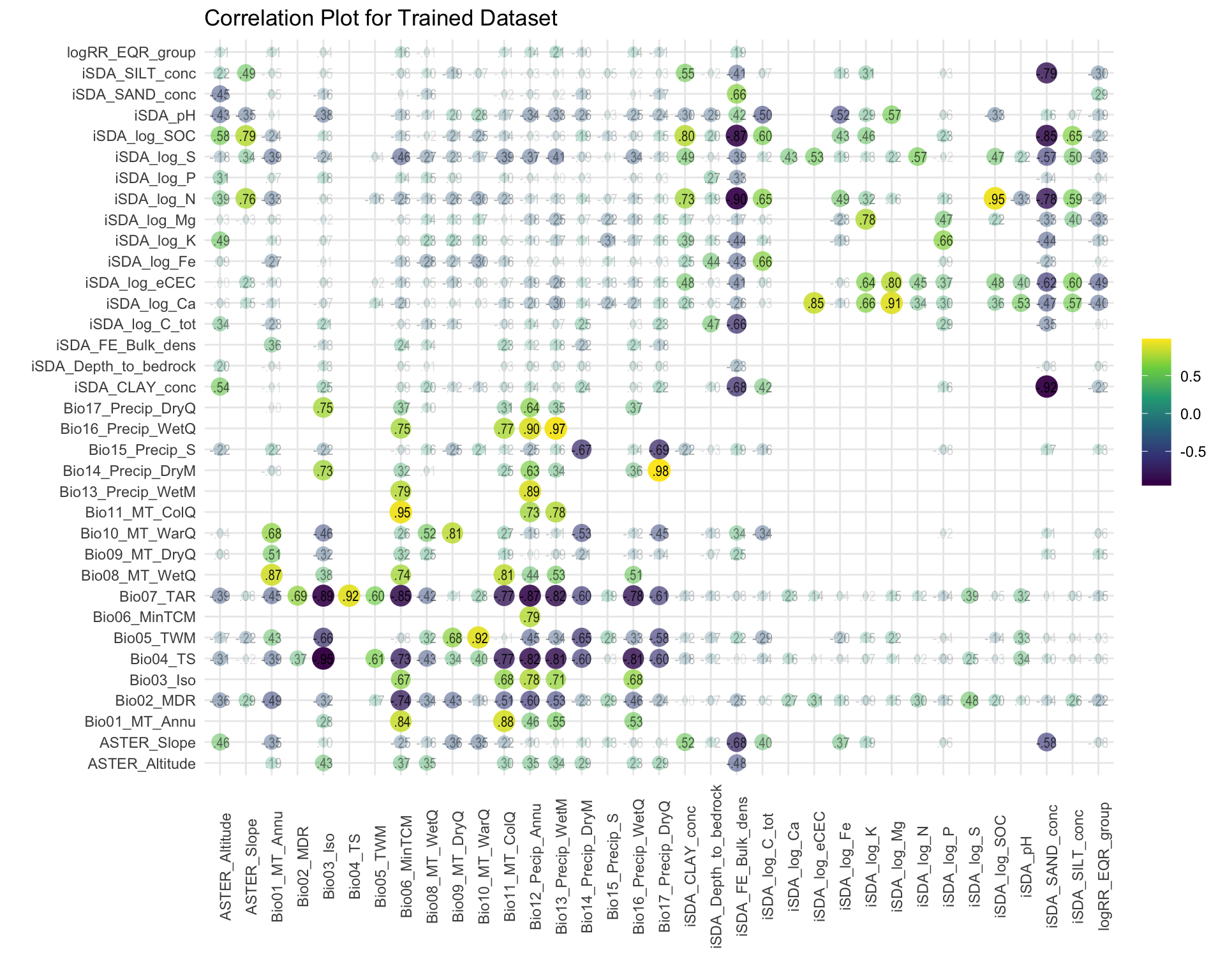
Figure 3: Correlation of variables against the EQR RR groups
STEP 8: Generate list of recipes
We generate a list of recipes for the Workflowset operations. The list consist of the recipes that wes generated earlier.
recipe_list <-
  list(normalize = normalize_recipe,
       removed_corr = rm_corr_recipe,
       interaction = interact_recipe)
STEP 7: Generate list of model types
We generate a list of model types for the Workflowset operations, as several model x recipe combinations will be tested. The model types are defined earlier when we defined our models.
model_list <-
list(Random_Forest = rf_mod,
     SVM = svm_mod,
     Naive_Bayes = nb_mod,
     Decision_Tree = dt_mod,
     Boosted_Trees = xgboost_mod,
     KNN = knn_mod,
     Logistic_Regression = logistic_mod)
STEP 8: Combine into a model Workflowset
Now we can combine the list of recipes and the list of models into a Workflowset - that we can use to tune.
model_set <- workflow_set(preproc = recipe_list,
                          models = model_list,
                          cross = T) # Setting cross = T instructs workflow_set to create all possible combinations of parsnip model and recipe specification.
STEP 9: Perform tuning of the model workflowsets
Now we can tune the Workflowset. Be aware that this operation can take around five hours on a standard laptop with 8 CPU, even when we use parallel processing.
Note that here we are using the tune_race_anuva() function/method to tune the Workflowset. There are other tuning methods available. We choose the tune_race_anova() because it is more efficient.
We define a control grid as a control aspects of the grid search racing process used in the Workflowset tuning.
race_ctrl_class <-
   control_race(
      save_pred = TRUE,
      parallel_over = "everything",
      save_workflow = TRUE
   )

set.seed(234)

# Initializing parallel processing
parallelStartSocket(cpus = detectCores())

wflwset_class_race_results <-
   model_set %>%
   workflow_map(fn        = "tune_race_anova",
                seed      = 3456,
                resamples = cv_fold,
                metrics   = multi.metric.class,
                verbose   = TRUE,
                grid      = 4,                       # simple and small grid
                control   = race_ctrl_class
   )

# Terminating parallel session
parallelStop()
We get a series of specific warning and error messages for various combinations of model-preprocessing, during the tuning, such as:
✓ 1 of 21 tuning: normalize_Random_Forest (4m 15.7s) i 2 of 21 tuning: normalize_SVM ! Fold4: internal: No observations were detected in truth for level(s): ‘1.extremely_low’ Computation will proceed by ignoring those levels.
✓ 6 of 21 tuning: normalize_KNN (3m 43.6s) i 7 of 21 tuning: normalize_Logistic_Regression x Fold4: preprocessor 1/1, model 1/4: Error: More than two classes; use multinomial family instead in call to glmnet x Fold4: preprocessor 1/1, model 2/4: Error: More than two classes; use multinomial family instead in call to glmnet
✓ 17 of 21 tuning: interaction_Naive_Bayes (3h 36m 10.5s) i 18 of 21 tuning: interaction_Decision_Tree ! Fold4: internal: No observations were detected in truth for level(s): ‘1.extremely_low’ Computation will proceed by ignoring those levels.
✓ 20 of 21 tuning: interaction_KNN (21m 19.2s) i 21 of 21 tuning: interaction_Logistic_Regression x Fold4: preprocessor 1/1, model 1/4: Error: More than two classes; use multinomial family instead in call to glmnet
SAVING THE WORKFLOWSET TUNING RESULTS
LOADING/READING THE WORKFLOWSET RESULTS
wflwset_class_race_results <- readRDS(here::here("TidyMod_Class_OUTPUT","wflwset_class_race_results.RDS"))
wflwset_class_race_results
# A workflow set/tibble: 21 × 4
   wflow_id                      info             option    result
   <chr>                         <list>           <list>    <list>
 1 normalize_Random_Forest       <tibble [1 × 4]> <opts[4]> <race[+]>
 2 normalize_SVM                 <tibble [1 × 4]> <opts[4]> <race[+]>
 3 normalize_Naive_Bayes         <tibble [1 × 4]> <opts[4]> <race[+]>
 4 normalize_Decision_Tree       <tibble [1 × 4]> <opts[4]> <race[+]>
 5 normalize_Boosted_Trees       <tibble [1 × 4]> <opts[4]> <race[+]>
 6 normalize_KNN                 <tibble [1 × 4]> <opts[4]> <race[+]>
 7 normalize_Logistic_Regression <tibble [1 × 4]> <opts[4]> <try-errr…
 8 removed_corr_Random_Forest    <tibble [1 × 4]> <opts[4]> <race[+]>
 9 removed_corr_SVM              <tibble [1 × 4]> <opts[4]> <race[+]>
10 removed_corr_Naive_Bayes      <tibble [1 × 4]> <opts[4]> <race[+]>
# … with 11 more rows
STEP 10: Cleaning op the Workflowsets
Cleaning op the Workflowsets so that the model-preprocessing combinations with errors are excluded
wflwset_class_race_results_clean <- wflwset_class_race_results %>%
  dplyr::filter(wflow_id != "normalize_Logistic_Regression",
                wflow_id != "removed_corr_Logistic_Regression",
                wflow_id != "interaction_Logistic_Regression")
Show code
autoplot(wflwset_class_race_results_clean)
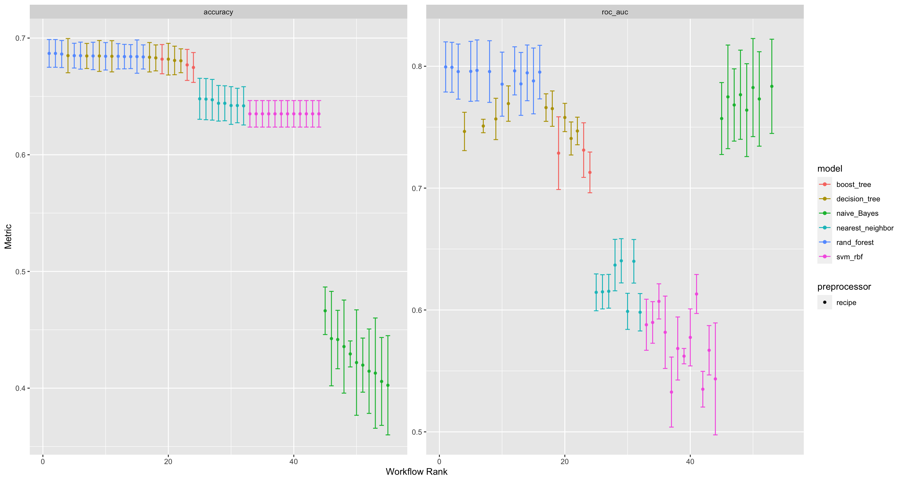
Figure 4: visualising the performances of the various model-preproccessing combinations
STEP 11: Evaluate performance of different model-preprocessing combinations
We can now evaluate, by visualising, the performance and compare the different Workflowsets.
Show code
workflowset_comparisons_accuracy <-
  collect_metrics(wflwset_class_race_results_clean) %>%
  separate(wflow_id, into = c("Recipe", "Model_Type"), sep = "_", remove = F, extra = "merge") %>%
  filter(.metric == "accuracy") %>%
  group_by(wflow_id) %>%
  filter(mean == max(mean)) %>%
  group_by(model) %>%
  dplyr::select(-.config) %>%
  distinct() %>%
  ungroup() %>%
  mutate(Workflow_Rank =  row_number(-mean),
         .metric = str_to_upper(.metric)) %>%
  ggplot(aes(x=Workflow_Rank, y = mean, shape = Recipe, color = Model_Type)) +
    geom_point() +
    geom_errorbar(aes(ymin = mean-std_err, ymax = mean+std_err)) +
    theme_minimal()+
    scale_colour_viridis_d() +
    labs(title = "Performance Comparison of Workflow Sets, metric: Accuracy", x = "Workflow Rank", y = "Accuracy", color = "Model Types", shape = "Recipes")

workflowset_comparisons_accuracy
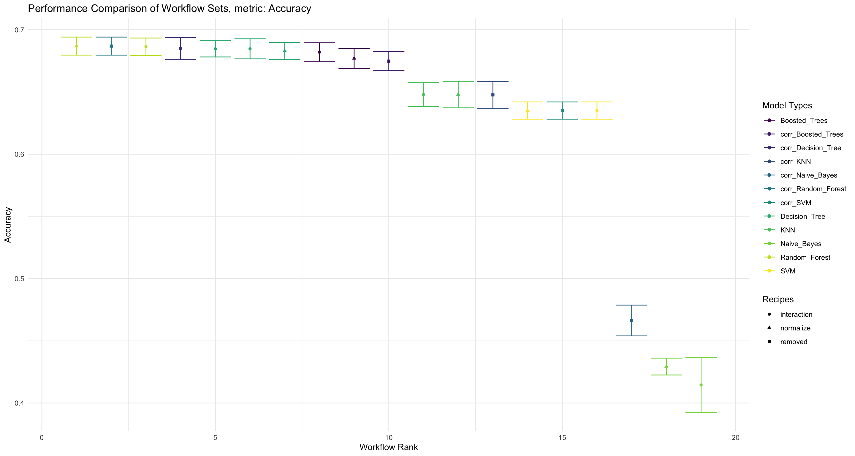
Figure 5: Evaluate the performance of accuracy and compare the different Workflowsets
We see that the Random Forest model with a normalized pre-processing recipe is the combination that performs the best, when looking at the Accuracy of the classification model.
Show code
workflowset_comparisons_aucroc <-
  collect_metrics(wflwset_class_race_results_clean) %>%
  separate(wflow_id, into = c("Recipe", "Model_Type"), sep = "_", remove = F, extra = "merge") %>%
  filter(.metric == "roc_auc") %>%
  group_by(wflow_id) %>%
  filter(mean == max(mean)) %>%
  group_by(model) %>%
  dplyr::select(-.config) %>%
  distinct() %>%
  ungroup() %>%
  mutate(Workflow_Rank =  row_number(-mean),
         .metric = str_to_upper(.metric)) %>%
  ggplot(aes(x=Workflow_Rank, y = mean, shape = Recipe, color = Model_Type)) +
    geom_point() +
    geom_errorbar(aes(ymin = mean-std_err, ymax = mean+std_err)) +
    theme_minimal()+
    scale_colour_viridis_d() +
    labs(title = "Performance Comparison of Workflow Sets, metric: AUC_ROC", x = "Workflow Rank", y = "ROC_AUC", color = "Model Types", shape = "Recipes")

workflowset_comparisons_aucroc
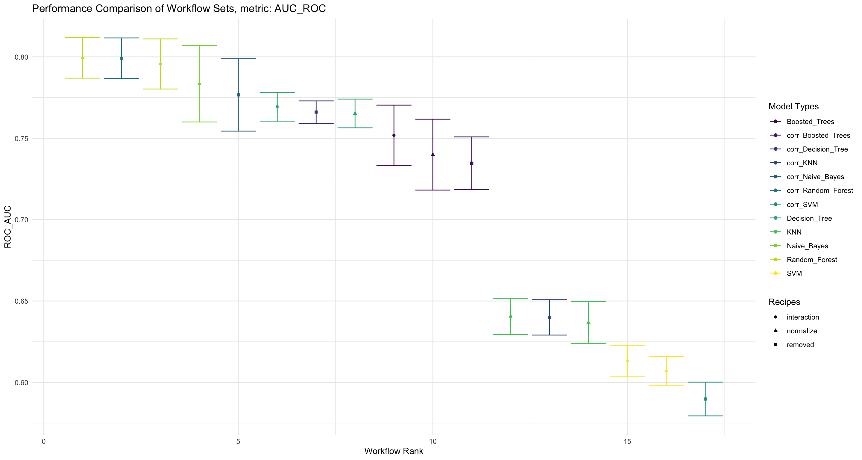
Figure 6: Evaluate the performance of AUC-ROC and compare the different Workflowsets
We see that the Random Forest model also performs best when it comes to the AUC_ROC metric.
STEP 12: List mode-preprocessing combinations
We can now list the Workflowset (model-preprocessing) combinations from best to worse, based on the AUC_ROC metric.
rank_results(wflwset_class_race_results_clean, rank_metric = "roc_auc", select_best = TRUE)
# A tibble: 34 × 9
   wflow_id   .config   .metric  mean std_err     n preprocessor model
   <chr>      <chr>     <chr>   <dbl>   <dbl> <int> <chr>        <chr>
 1 normalize… Preproce… accura… 0.687 0.00723     5 recipe       rand…
 2 normalize… Preproce… roc_auc 0.799 0.0125      5 recipe       rand…
 3 removed_c… Preproce… accura… 0.687 0.00723     5 recipe       rand…
 4 removed_c… Preproce… roc_auc 0.799 0.0125      5 recipe       rand…
 5 interacti… Preproce… accura… 0.685 0.00714     5 recipe       rand…
 6 interacti… Preproce… roc_auc 0.796 0.0154      5 recipe       rand…
 7 normalize… Preproce… accura… 0.413 0.0287      5 recipe       naiv…
 8 normalize… Preproce… roc_auc 0.784 0.0235      5 recipe       naiv…
 9 removed_c… Preproce… accura… 0.436 0.0242      5 recipe       naiv…
10 removed_c… Preproce… roc_auc 0.777 0.0222      5 recipe       naiv…
# … with 24 more rows, and 1 more variable: rank <int>
The Random Forest model is clearly the winner! It performs best on all the pre-processing recipeis. The Random Forest is closely followed by the Naive_Bayes models.
STEP 13: Finalize worfkflow with best model
We can now finalize the Workflowset with the best performing workflow (model-preprocessing combinations)
Get the best parameters and finalize
#Pull Best Performing Hyperparameter Set From workflow_map Object
best_result <- wflwset_class_race_results_clean %>%
  pull_workflow_set_result("normalize_Random_Forest") %>%
  select_best(metric = "accuracy")
#Finalise Workflow Object With Best Parameters
dt_wf <- wflwset_class_race_results_clean %>%
  pull_workflow("normalize_Random_Forest") %>%
  finalize_workflow(best_result)

#Fit Workflow Object to Training Data and Predict Using Testing Dataset

dt_res <-
  dt_wf %>%
  fit(training(af.split.class)) %>%
  predict(new_data = testing(af.split.class)) %>%
  bind_cols(af.test.class) %>%
  mutate(.pred_class = fct_infreq(.pred_class),
         logRR_EQR_group = fct_infreq(logRR_EQR_group)) %>%
  rationalize() %>%
  drop_na() %>%
  relocate(logRR_EQR_group, .pred_class)

dt_res
# A tibble: 884 × 45
   logRR_EQR_group .pred_class PrName    Out.SubInd  Product Site.Type
   <fct>           <fct>       <fct>     <fct>       <fct>   <fct>
 1 4.medium        4.medium    Parklands Biomass Yi… Pearl … Farm
 2 4.medium        5.high      Agrofore… Biomass Yi… Pearl … Farm
 3 4.medium        5.high      Agrofore… Crop Yield  Pearl … Farm
 4 4.medium        4.medium    Agrofore… Crop Yield  Pearl … Station
 5 4.medium        4.medium    Agrofore… Biomass Yi… Maize   Station
 6 5.high          4.medium    Agrofore… Crop Yield  Maize   Station
 7 4.medium        4.medium    Agrofore… Biomass Yi… Maize   Station
 8 4.medium        4.medium    Alleycro… Crop Yield  Maize   Farm
 9 4.medium        4.medium    Agrofore… Crop Yield  Maize   Farm
10 4.medium        4.medium    Agrofore… Crop Yield  Maize   Farm
# … with 874 more rows, and 39 more variables: Tree <fct>,
#   Out.SubInd.Code <fct>, Latitude <dbl>, Longitude <dbl>,
#   Bio01_MT_Annu <dbl>, Bio02_MDR <dbl>, Bio03_Iso <dbl>,
#   Bio04_TS <dbl>, Bio05_TWM <dbl>, Bio06_MinTCM <dbl>,
#   Bio07_TAR <dbl>, Bio08_MT_WetQ <dbl>, Bio09_MT_DryQ <dbl>,
#   Bio10_MT_WarQ <dbl>, Bio11_MT_ColQ <dbl>, Bio12_Pecip_Annu <dbl>,
#   Bio13_Precip_WetM <dbl>, Bio14_Precip_DryM <dbl>, …
By visualising the modelled RR groups in a correlation plot we see that the predicted () RR groups are correlated mostly with precipitation of the dry quarter Magnanimous etc.
Show code
  coor_plot_EQR_modelled <-
  dt_res %>%
  dplyr::select(-c(PrName, Out.SubInd, Product, Site.Type, Tree, Out.SubInd.Code)) %>%
  mutate(.pred_class = if_else(.pred_class == "5.high", 1,0)) %>%
  dplyr::select(2:38) %>%
              correlate() %>%
              rearrange() %>%
              shave() %>%
              rplot(print_cor = T,.order = "alphabet") +
                theme_minimal() +
                theme(axis.text.x = element_text(angle = 90)) +
                scale_color_viridis_c() +
                labs(title = "Correlation Plot for Testing Dataset - modelled")

coor_plot_EQR_modelled
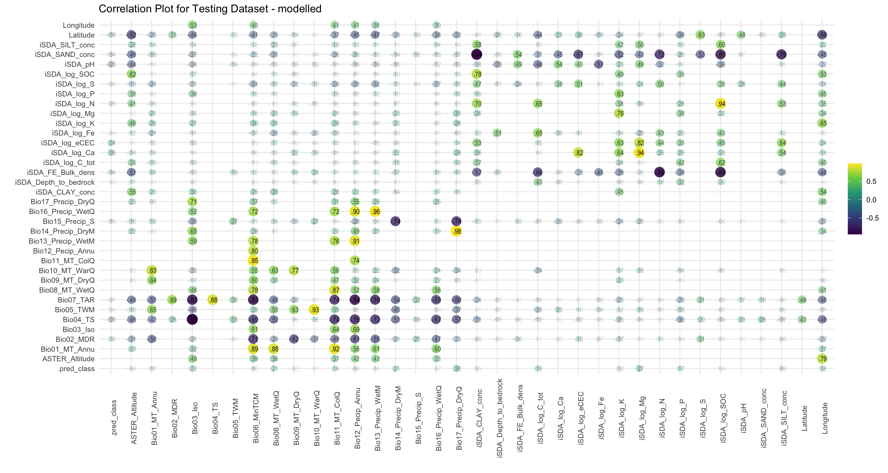
Figure 7: Correlation of variables against the modelled EQR RR groups
STEP 14: Generate confusion matrix of predicted vs observed RR groups
Show code
final_param <-
  wflwset_class_race_results_clean %>%
  pull_workflow_set_result("normalize_Random_Forest") %>%
  show_best("roc_auc") %>%
  dplyr::slice(1) %>%
  dplyr::select(trees, mtry)

wflwset_class_race_results_clean %>%
  pull_workflow_set_result("normalize_Random_Forest") %>%
  collect_predictions() %>%
  inner_join(final_param) %>%
  group_by(id) %>%
  conf_mat(truth = logRR_EQR_group, estimate = .pred_class) %>%
  mutate(tidied = map(conf_mat, tidy)) %>%
  unnest(tidied)
# A tibble: 245 × 4
   id    conf_mat   name     value
   <chr> <list>     <chr>    <int>
 1 Fold1 <conf_mat> cell_1_1     0
 2 Fold1 <conf_mat> cell_2_1     0
 3 Fold1 <conf_mat> cell_3_1     0
 4 Fold1 <conf_mat> cell_4_1     1
 5 Fold1 <conf_mat> cell_5_1     0
 6 Fold1 <conf_mat> cell_6_1     0
 7 Fold1 <conf_mat> cell_7_1     0
 8 Fold1 <conf_mat> cell_1_2     0
 9 Fold1 <conf_mat> cell_2_2     0
10 Fold1 <conf_mat> cell_3_2     1
# … with 235 more rows
Confusion matrix of predicted vs observed RR groups
                  Truth
Prediction         1.extremely_low 2.very_low 3.low 4.medium 5.high
  1.extremely_low                0          0     0        0      0
  2.very_low                     0          0     0        0      0
  3.low                          3          5    36       36      1
  4.medium                       7         29   172     2074    534
  5.high                         0          4    18      207    385
  6.very_high                    0          0     0        1      7
  7.extremely_high               0          0     0        0      1
                  Truth
Prediction         6.very_high 7.extremely_high
  1.extremely_low            0                0
  2.very_low                 0                0
  3.low                      0                0
  4.medium                  69               11
  5.high                    37                1
  6.very_high               12                0
  7.extremely_high           0                0
As we see the classes are highly unbalanced and this makes it “difficult” for the Random Forest model (or any model) to create robust predictions. A way to circumvent this is to use the pre-processing steps from the themis package. The themis package is specifically designed for optimizing machine learning classification modelling by providing extra pre-processing reccipe steps for unbalanced data. themis (https://github.com/tidymodels/themis) contains extra steps for the recipes package for dealing with unbalanced data. The name themis is that of the ancient Greek god who is typically depicted with a balance.
Show code
autoplot(conf_matrix, type = "mosaic")
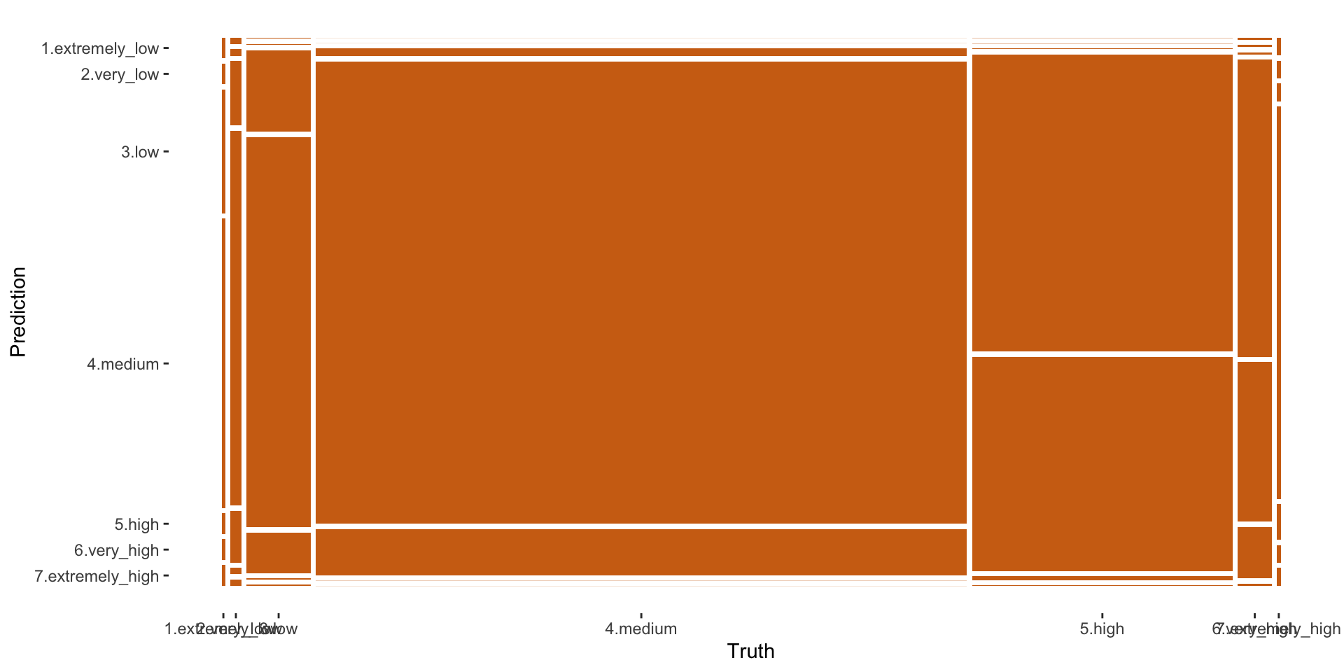
Figure 8: Printing confusion matrix - mosaic
Show code
autoplot(conf_matrix, type = "heatmap")
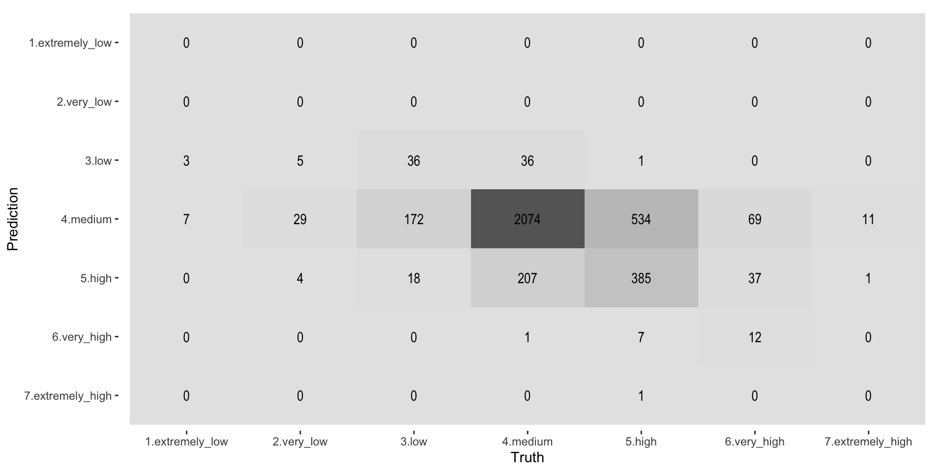
Figure 9: Printing confusion matrix - heatmap