Here we are going to explore Machine Learning with Tidymodels on the ERA agroforestry data
These objects can be created by crossing all combinations of pre-processors (e.g., formula, recipe, etc) and model specifications. This different model toolkit in the arsenal of
Loading necessary R packages and ERA data
Loading general R packages
This part of the document is where we actually get to the nitty-gritty of the ERA agroforestry data and therefore it requires us to load a number of R packages for both general Explorortive Data Analysis and Machine Learning.
Show code
# Using the pacman functions to load required packages

        if(!require("pacman", character.only = TRUE)){
          install.packages("pacman",dependencies = T)
          }

# ------------------------------------------------------------------------------------------
# General packages
# ------------------------------------------------------------------------------------------
required.packages <- c("tidyverse", "tidymodels", "finetune", "kernlab", "here", "hablar", "spatialsample", "cowplot",
                       "stacks", "rules", "baguette", "viridis", "yardstick", "DALEXtra", "see", "ggridges",
# ------------------------------------------------------------------------------------------
# Parallel computing packages
# ------------------------------------------------------------------------------------------
                      "parallelMap", "parallelly", "parallel", "doParallel"
)

p_load(char=required.packages, install = T,character.only = T)
STEP 1: Getting the data
Removing outliers from logRR
is_outlier <- function(x) {
  return(x < quantile(x, 0.25) - 3 * IQR(x) | x > quantile(x, 0.75) + 3 * IQR(x))
}

ml.data.outliers.wf <- ml.data.wf %>%
  rationalize(logRR) %>%
  drop_na(logRR) %>%
  mutate(ERA_Agroforestry = 1) %>%
  group_by(ERA_Agroforestry) %>%
  mutate(logRR.outlier = ifelse(is_outlier(logRR), logRR, as.numeric(9999))) %>%
  ungroup()
Agroforestry data with no outliers
Notice we do not remove missing values
STEP 2: Splitting data
Split data in training and testing sets
set.seed(456)

# Splitting data
af.split.wf <- initial_split(ml.data.no.outliers.wf, prop = 0.80, strata = logRR)

af.train.wf <- training(af.split.wf)
af.test.wf <- testing(af.split.wf)
STEP 3: Define resampling techniques on training data
Notice here that we do not have any repeats defined as we did originally. Previously we used an argument: repeats = 10 to specify the number of times to repeat the V-fold partitioning. Instead we are increasing the number of partitions/folds (v) from 10 to 20, for the cv-folds, just as the spatial clustering cv-folds.
STEP 4: Define model metrics
STEP 5: Create pre-processing recipies
base_recipe <-
  recipe(formula = logRR ~ ., data = af.train.wf) %>%
  update_role(Site.Type, new_role = "predictor") %>% # alters an existing role in the recipe to variables.
  update_role(PrName, # or assigns an initial role to variables that do not yet have a declared role.
              Out.SubInd,
              Out.SubInd.Code,
              Product,
              Latitude,
              Longitude,
              Tree,
              new_role = "sample ID")
# ------------------------------------------------------------------------------------------------------------------------------------------------


impute_mean_recipe <-
  base_recipe %>%
  step_impute_mean(all_numeric_predictors(), skip = FALSE) %>%
  step_novel(Site.Type, skip = FALSE) %>%
  step_dummy(Site.Type, one_hot = TRUE, naming = partial(dummy_names,sep = "_"), skip = FALSE) %>%
  step_zv(all_predictors(), skip = FALSE) %>% # remove any columns with a single unique value
  step_nzv(all_predictors(), skip = FALSE)


impute_knn_recipe <-
  base_recipe %>%
  step_impute_knn(all_numeric_predictors(), skip = FALSE) %>%
  step_novel(Site.Type, skip = FALSE) %>%
  step_dummy(Site.Type, one_hot = TRUE, naming = partial(dummy_names,sep = "_"), skip = FALSE) %>%
  step_zv(all_predictors(), skip = FALSE) %>% # remove any columns with a single unique value
  step_nzv(all_predictors(), skip = FALSE)


normalize_recipe <-
  base_recipe %>%
  step_impute_linear(all_numeric_predictors(), impute_with = imp_vars(Longitude, Latitude), skip = FALSE) %>% # create linear regression models to impute missing data.
  step_novel(Site.Type, skip = FALSE) %>%
  step_dummy(Site.Type, one_hot = TRUE, naming = partial(dummy_names,sep = "_"), skip = FALSE) %>%
  step_zv(all_predictors(), skip = FALSE) %>% # remove any columns with a single unique value
  step_nzv(all_predictors(), skip = FALSE) %>%
  step_normalize(all_numeric_predictors(), skip = FALSE) # normalize numeric data: standard deviation of one and a mean of zero.

rm_corr_recipe <-
  base_recipe %>%
  step_impute_linear(all_numeric_predictors(), impute_with = imp_vars(Longitude, Latitude), skip = FALSE) %>% # create linear regression models to impute missing data.
  step_novel(Site.Type, skip = FALSE) %>%
  step_dummy(Site.Type, one_hot = TRUE, naming = partial(dummy_names,sep = "_"), skip = FALSE) %>%
  step_zv(all_predictors(), skip = FALSE) %>% # remove any columns with a single unique value
  step_nzv(all_predictors(), skip = FALSE) %>%
  step_corr(all_numeric_predictors(), threshold = 0.8, method = "pearson", skip = FALSE)

interact_recipe <-
  base_recipe %>%
  step_impute_linear(all_numeric_predictors(), impute_with = imp_vars(Longitude, Latitude), skip = FALSE) %>% # create linear regression models to impute missing data.
  step_novel(Site.Type, skip = FALSE) %>%
  step_dummy(Site.Type, one_hot = TRUE, naming = partial(dummy_names,sep = "_"), skip = FALSE) %>%
  step_zv(all_predictors(), skip = FALSE) %>% # remove any columns with a single unique value
  step_nzv(all_predictors(), skip = FALSE) %>%
  step_interact(~ all_numeric_predictors():all_numeric_predictors(), skip = FALSE)
Note: To view how the recipe pre-process the data simply pipe it into a prep() function to prepare it, then a juice() function to extract it and then its a good idea to make use of the glimpse() function to easily see each variable.
STEP 6: Defining model specifications
lm_spec <- linear_reg() %>%
  set_mode("regression") %>%
  set_engine("lm")

glm_spec <- linear_reg(
  penalty = tune(),
  mixture = tune()) %>%
  set_engine("glmnet") %>%
  set_mode("regression")

cart_spec <-
   decision_tree(cost_complexity = tune(),
                 min_n = tune()) %>%
   set_engine("rpart") %>%
   set_mode("regression")

mars_spec <-
   mars(prod_degree = tune()) %>%  #<- use GCV to choose terms
   set_engine("earth") %>%
   set_mode("regression")

knn_spec <-
   nearest_neighbor(neighbors = tune(),
                    weight_func = tune()) %>%
   set_engine("kknn") %>%
   set_mode("regression")

svm_p_spec <-
   svm_poly(cost = tune(),
            degree = tune()) %>%
   set_engine("kernlab") %>%
   set_mode("regression")

cubist_spec <-
   cubist_rules(committees = tune(),
                neighbors = tune()) %>%
   set_engine("Cubist")

nnet_spec <-
   mlp(hidden_units = tune(),
       penalty = tune(),
       epochs = tune()) %>%
   set_engine("nnet", MaxNWts = 2600) %>%
   set_mode("regression")

rf_spec <-
   rand_forest(mtry = tune(),
               min_n = tune(),
               trees = tune()) %>%
   set_engine("ranger") %>%
   set_mode("regression")

xgb_spec <-
   boost_tree(tree_depth = tune(),
              learn_rate = tune(),
              loss_reduction = tune(),
              min_n = tune(),
              sample_size = tune(),
              trees = tune()) %>%
   set_engine("xgboost") %>%
   set_mode("regression")
STEP 7: Integrating pre-processing and model specification into a workflowset
wflwset_setup <-
   workflow_set(
      preproc = list(impute_mean = impute_mean_recipe,
                     impute_knn = impute_knn_recipe,
                     normalized = normalize_recipe,
                     rm_corr = rm_corr_recipe,
                     interaction = interact_recipe),
      models = list(lm = lm_spec,
                    glm = glm_spec,
                    cart = cart_spec,
                    mars = mars_spec,
                    knn = knn_spec,
                    svm_p = svm_p_spec,
                    cubist = cubist_spec,
                    nnet = nnet_spec,
                    RF = rf_spec,
                    XGB = xgb_spec),
      cross = TRUE
   )

saveRDS(wflwset_setup, file = here::here("TidyModWflSet_OUTPUT", "wflwset_setup.RDS"))
# A workflow set/tibble: 50 × 4
   wflow_id           info             option    result
   <chr>              <list>           <list>    <list>
 1 impute_mean_lm     <tibble [1 × 4]> <opts[0]> <list [0]>
 2 impute_mean_glm    <tibble [1 × 4]> <opts[0]> <list [0]>
 3 impute_mean_cart   <tibble [1 × 4]> <opts[0]> <list [0]>
 4 impute_mean_mars   <tibble [1 × 4]> <opts[0]> <list [0]>
 5 impute_mean_knn    <tibble [1 × 4]> <opts[0]> <list [0]>
 6 impute_mean_svm_p  <tibble [1 × 4]> <opts[0]> <list [0]>
 7 impute_mean_cubist <tibble [1 × 4]> <opts[0]> <list [0]>
 8 impute_mean_nnet   <tibble [1 × 4]> <opts[0]> <list [0]>
 9 impute_mean_RF     <tibble [1 × 4]> <opts[0]> <list [0]>
10 impute_mean_XGB    <tibble [1 × 4]> <opts[0]> <list [0]>
# … with 40 more rows
We see very clearly that a workflowset contains all possible combinations of model specifications and pre-processing steps. A powerful way to test several models on different forms of pre-processing specifications to scan and find the best setup.
STEP 8: Tuning workflowsets using tune_grid() or tune_race_anova()
There are different ways we can tune/fit our workflowsets. The more traditional one is using tune_grid() from the tune package, that is part of tidymodels. With tune_grid() we will compute a set of performance metrics (e.g. MAE or RMSE) for a pre-defined set of tuning parameters that correspond to a model or recipe across one or more resamples of the data. Hence all set combinations of (hyper)-parameters for the models are used to tune the models individually. This can sometimes cause really long and expensive model tuning.
A more effecient alternative to tune_grid() is the tune_race_anova() from the finetune package. Instead of tuning the individual models based on all possible combinations of (hyper)-parameters tune_race_anova() computes a set of performance metrics (e.g. MAE or RMSE) for a pre-defined set of tuning parameters that correspond to a model or recipe across one or more resamples of the data. After an initial number of resamples have been evaluated, the process eliminates tuning parameter combinations that are unlikely to be the best results using a repeated measure ANOVA model. This approach is significantly more efficient, as not all (hyper)-parameter combination will have to be used in the model tuning process, but only the ones that in a step-wise manner improve model performance.
Using tune_grid()
Note: we are not going to do this because it takes too long
#  # Initializing parallel processing
#  doParallel::registerDoParallel()
#
# set.seed(123)
#
# wflwset_setup_res <-
#    wflwset_setup %>%
#    # The first argument is a function name from the {{tune}} package such as `tune_grid()`, `fit_resamples()`, etc.
#    workflow_map(fn        = "tune_grid",
#                 resamples = cv.fold.wf,
#                 grid      = 5,
#                 metrics   = multi.metric.wf,
#                 verbose   = TRUE)
#
# # Terminating parallel session
# parallelStop()
Using tune_race_anova()
Note: More than 50 model-pre-processing combinations have to be tuned. This tuning takes about 5 hours with a normal 8 CPU computer - even when running in parallel.
The tune_race_anove() uses an innovative method to speed up the tuning of machine learning models. tune_race_anova() computes a set of performance metrics (e.g. accuracy or RMSE) for a pre-defined set of tuning parameters that correspond to a model or recipe across one or more resamples of the data. After an initial number of resamples have been evaluated, the process eliminates tuning parameter combinations that are unlikely to be the best results using a repeated measure ANOVA model.
race_ctrl <-
   control_race(
      save_pred = TRUE,
      parallel_over = "everything",
      save_workflow = TRUE
   )

 # Initializing parallel processing
 doParallel::registerDoParallel()

wflwset_setup_race_results <-
   wflwset_setup %>%
   workflow_map(fn        = "tune_race_anova",
                seed      = 1503,
                resamples = cv.fold.wf,
                metrics   = multi.metric.wf,
                verbose   = TRUE,
                grid      = 5,
                control   = race_ctrl
   )

# Terminating parallel session
parallelStop()
There are some model - pre-processing combinations that do not successfully manage to get tuned:
i 46 of 50 tuning: interaction_svm_p Warning in mclapply(argsList, FUN, mc.preschedule = preschedule, mc.set.seed = set.seed, : scheduled core 2 did not deliver a result, all values of the job will be affected x 46 of 50 tuning: interaction_svm_p failed with: Error in contrasts<-(*tmp*, value = contr.funs[1 + isOF[nn]]) : contrasts can be applied only to factors with 2 or more levels i 47 of 50 tuning: interaction_cubist ✓ 47 of 50 tuning: interaction_cubist (21m 26s) i 48 of 50 tuning: interaction_nnet x 48 of 50 tuning: interaction_nnet failed with: Error in contrasts<-(*tmp*, value = contr.funs[1 + isOF[nn]]) : contrasts can be applied only to factors with 2 or more levels i 49 of 50 tuning: interaction_RF i Creating pre-processing data to finalize unknown parameter: mtry ✓ 49 of 50 tuning: interaction_RF (1h 33m 57.8s) i 50 of 50 tuning: interaction_XGB ✓ 50 of 50 tuning: interaction_XGB (31m 33.5s)
We will have to delete these from the output.
SAVING THE WORKFLOWSET TUNING RESULTS
STEP 9: Assessing results of the tuned workflowsets
From tune_grid()
Show code
# -------------------------------------------------------------------
# LOAD THE TUNED (tune_race_anova) WORKFLOWSET DATA

wflwset_setup_race_results <- readRDS(here::here("TidyModWflSet_OUTPUT", "wflwset_setup_race_results.RDS"))
#Error: There were 1 workflows that had no results.

# Removing the result that caused the error for not having a result

wflwset_setup_race_results_clean <- wflwset_setup_race_results %>%
  dplyr::filter(wflow_id != "interaction_svm_p")  %>%
  dplyr::filter(wflow_id != "interaction_nnet")

saveRDS(wflwset_setup_race_results_clean, here::here("TidyModWflSet_OUTPUT","wflwset_setup_race_results_clean.RDS"))
Show code
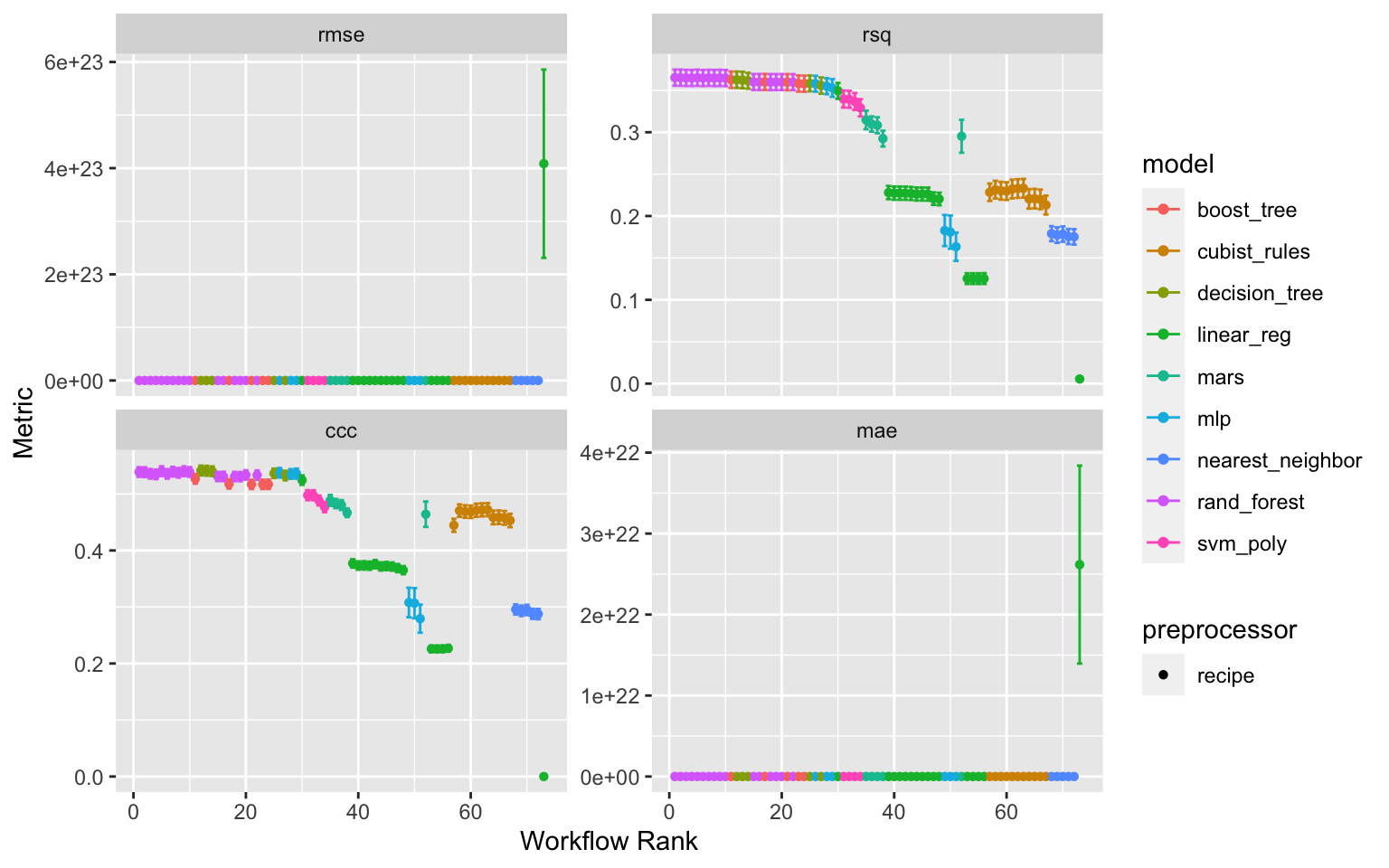
Figure 1: Results of the tune race anova workflowset tuning
Show code
wflwset_setup_race_results_clean_no_linear <- wflwset_setup_race_results_clean %>%
  dplyr::filter(!str_detect(wflow_id, "_lm"))

autoplot(wflwset_setup_race_results_clean_no_linear)
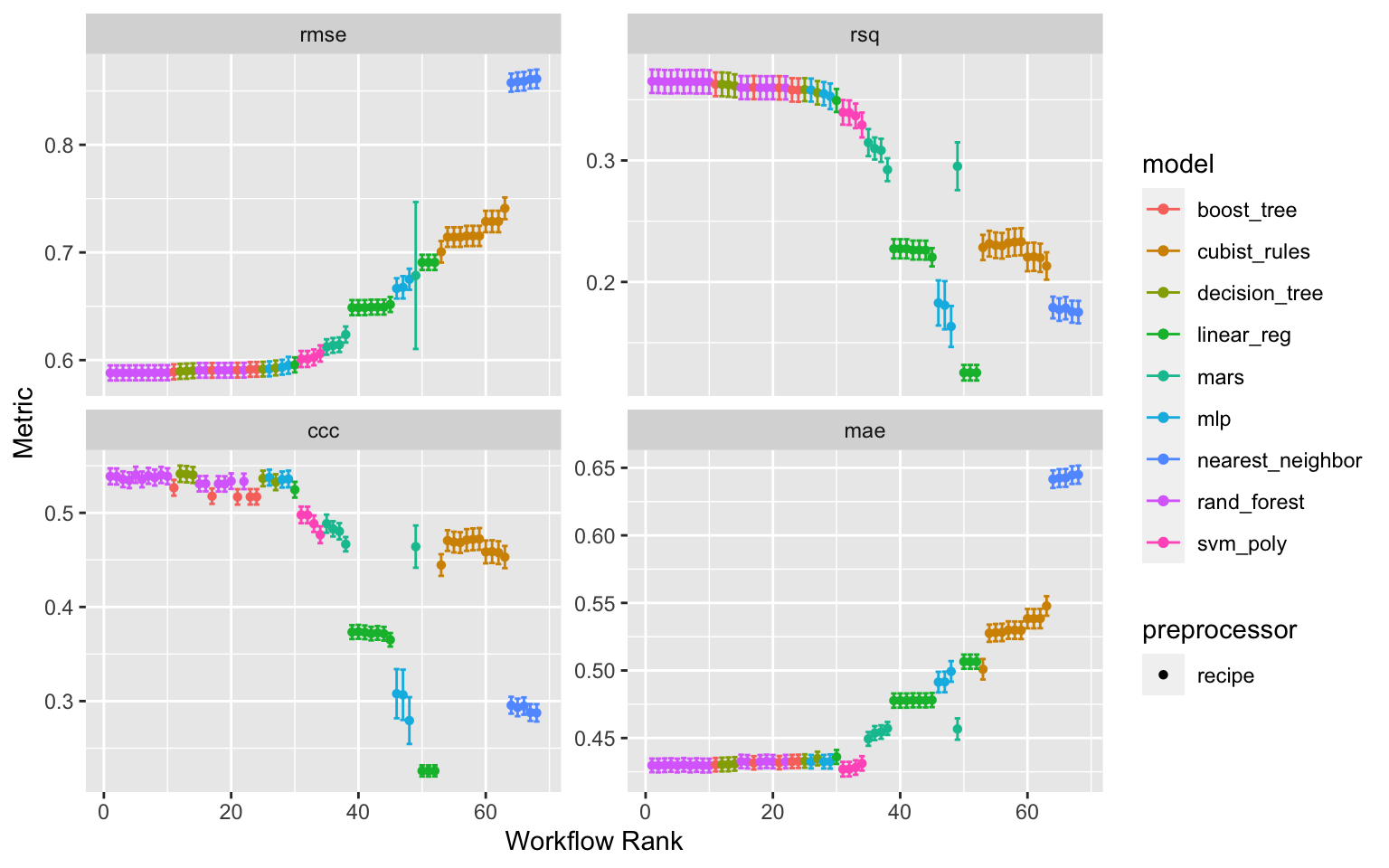
Figure 2: Results of the tune race anova workflowset tuning after lm models have been excluded
Ranking Workflowsets results from model-pre-processing combinations
First removing the linear models, that seems unrealistically poor in predicting the response ratios. The ranking is done for the two metrics; RMSE and CCC
rank_results(wflwset_setup_race_results_clean_no_linear,
             rank_metric = "rmse",
             select_best = TRUE) %>%
  select(rank, mean, model, wflow_id, .config) %>%
  arrange(desc(-rank))
# A tibble: 172 × 5
    rank  mean model       wflow_id       .config
   <int> <dbl> <chr>       <chr>          <chr>
 1     1 0.539 rand_forest normalized_RF  Preprocessor1_Model5
 2     1 0.430 rand_forest normalized_RF  Preprocessor1_Model5
 3     1 0.588 rand_forest normalized_RF  Preprocessor1_Model5
 4     1 0.365 rand_forest normalized_RF  Preprocessor1_Model5
 5     2 0.539 rand_forest rm_corr_RF     Preprocessor1_Model5
 6     2 0.430 rand_forest rm_corr_RF     Preprocessor1_Model5
 7     2 0.588 rand_forest rm_corr_RF     Preprocessor1_Model5
 8     2 0.365 rand_forest rm_corr_RF     Preprocessor1_Model5
 9     3 0.537 rand_forest interaction_RF Preprocessor1_Model2
10     3 0.430 rand_forest interaction_RF Preprocessor1_Model2
# … with 162 more rowsrank_results(wflwset_setup_race_results_clean_no_linear,
rank_metric = "ccc",
select_best = TRUE) %>%
select(rank, mean, model, wflow_id, .config) %>%
arrange(desc(-rank))
# A tibble: 172 × 5
    rank  mean model         wflow_id        .config
   <int> <dbl> <chr>         <chr>           <chr>
 1     1 0.541 decision_tree normalized_cart Preprocessor1_Model2
 2     1 0.430 decision_tree normalized_cart Preprocessor1_Model2
 3     1 0.590 decision_tree normalized_cart Preprocessor1_Model2
 4     1 0.363 decision_tree normalized_cart Preprocessor1_Model2
 5     2 0.541 decision_tree rm_corr_cart    Preprocessor1_Model2
 6     2 0.430 decision_tree rm_corr_cart    Preprocessor1_Model2
 7     2 0.590 decision_tree rm_corr_cart    Preprocessor1_Model2
 8     2 0.362 decision_tree rm_corr_cart    Preprocessor1_Model2
 9     3 0.540 rand_forest   normalized_RF   Preprocessor1_Model4
10     3 0.430 rand_forest   normalized_RF   Preprocessor1_Model4
# … with 162 more rows
STEP 10: Finalizing models
Similar to what we went through in Part 3: Analysing with Tidymodels, we also have to finalize the models from the tuning results using the best performing (hyper)-parameter configurations. We are going to do this last fitting of the models using the training set. The first step is to pick a workflow to finalize. Since Random Forest models (RF), boosted tree models (XGB), decision tree models (cart) and generalized linear models (glm) worked well, we’ll extract the best configurations from the sets, update the parameters with the numerically best settings, and fit to the training set.
Extracting best performing model (hyper)-parameter configurations
rf_wf_best_rmse_results_of_race <-
   wflwset_setup_race_results_clean %>%
   extract_workflow_set_result("normalized_RF") %>%
   select_best(metric = "rmse")

xgb_wf_best_rmse_results_of_race <-
   wflwset_setup_race_results_clean %>%
   extract_workflow_set_result("interaction_XGB") %>%
   select_best(metric = "rmse")

cart_wf_best_rmse_results_of_race <-
   wflwset_setup_race_results_clean %>%
   extract_workflow_set_result("rm_corr_cart") %>%
   select_best(metric = "rmse")

glm_wf_best_rmse_results_of_race <-
   wflwset_setup_race_results_clean %>%
   extract_workflow_set_result("interaction_glm") %>%
   select_best(metric = "rmse")
Saving best performing models
Show code
# SAVING THE BEST PERFORMING MODEL CONFIGURATIONS

saveRDS(rf_wf_best_rmse_results_of_race, here::here("TidyModWflSet_OUTPUT","rf_wf_best_rmse_results_of_race.RDS"))
saveRDS(xgb_wf_best_rmse_results_of_race, here::here("TidyModWflSet_OUTPUT","xgb_wf_best_rmse_results_of_race.RDS"))
saveRDS(cart_wf_best_rmse_results_of_race, here::here("TidyModWflSet_OUTPUT","cart_wf_best_rmse_results_of_race.RDS"))
saveRDS(glm_wf_best_rmse_results_of_race, here::here("TidyModWflSet_OUTPUT","glm_wf_best_rmse_results_of_race.RDS"))
Performing last fitting on the whole dataset (traningset + testingset)
rf_best_race_last_fit <-
   wflwset_setup_race_results_clean %>%
   extract_workflow("normalized_RF") %>%
   finalize_workflow(rf_wf_best_rmse_results_of_race) %>%
   last_fit(split = af.split.wf)

xgb_best_race_last_fit <-
   wflwset_setup_race_results_clean %>%
   extract_workflow("interaction_XGB") %>%
   finalize_workflow(xgb_wf_best_rmse_results_of_race) %>%
   last_fit(split = af.split.wf)

cart_best_race_last_fit <-
   wflwset_setup_race_results_clean %>%
   extract_workflow("rm_corr_cart") %>%
   finalize_workflow(cart_wf_best_rmse_results_of_race) %>%
   last_fit(split = af.split.wf)

glm_best_race_last_fit <-
   wflwset_setup_race_results_clean %>%
   extract_workflow("interaction_glm") %>%
   finalize_workflow(glm_wf_best_rmse_results_of_race) %>%
   last_fit(split = af.split.wf)
Saving last fitting results of models
Show code
# SAVING THE BEST PERFORMING MODEL CONFIGURATIONS

saveRDS(rf_best_race_last_fit, here::here("TidyModWflSet_OUTPUT","rf_best_race_last_fit.RDS"))
saveRDS(xgb_best_race_last_fit, here::here("TidyModWflSet_OUTPUT","xgb_best_race_last_fit.RDS"))
saveRDS(cart_best_race_last_fit, here::here("TidyModWflSet_OUTPUT","cart_best_race_last_fit.RDS"))
saveRDS(glm_best_race_last_fit, here::here("TidyModWflSet_OUTPUT","glm_best_race_last_fit.RDS"))
STEP 11: Assessing/evaluating model performance
Viewing the performance of the Random Forest model for RMSE and rsq
Show code
# A tibble: 2 × 4
  .metric .estimator .estimate .config
  <chr>   <chr>          <dbl> <chr>
1 rmse    standard       0.600 Preprocessor1_Model1
2 rsq     standard       0.393 Preprocessor1_Model1
Contructing predicted vs observed plot for the Random Forest
Show code
rf_wflowset_last_fit_plot <-
  rf_best_race_last_fit %>%
  collect_predictions() %>%
  ggplot(aes(x = logRR, y = .pred)) +
  geom_abline(col = "red", lty = 2) +
  #geom_smooth(method = "gam", linetype = "dashed", col = "black", size = 1) +
  geom_jitter(width = 0.5, height = 0.2, alpha = 0.5) +
  coord_obs_pred(ratio = 1.2) +
  labs(x = "Observed RR (log scale)", y = "Predicted RR (log scale)")
Show code
rf_wflowset_last_fit_plot
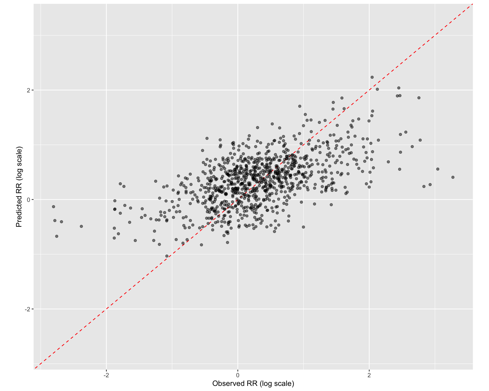
Figure 3: Prediccted vs observed for the Random Forest model
Listing some predicted vs observed values of response ratios
Show code
rmarkdown::paged_table(

rf_best_race_last_fit %>%
  collect_predictions() %>%
  arrange(desc(.pred))

)
STEP 12: Explaining models and predictions (model agnostics) with local break-down plots
We suggested that model performance, as measured by appropriate metrics (like RMSE for regression or area under the ROC curve for classification), can be important for all applications of modelling. Similarly, model explanations, answering why a model makes the predictions it does, can be important whether the purpose of your model is largely descriptive, to test a hypothesis, or to make a prediction. Answering the question “why?” allows modelling practitioners to understand which features were important in predictions and even how model predictions would change under different values for the features.
For some models, like linear regression, it is usually clear how to explain why the model makes the predictions it does. The structure of a linear model contains coefficients for each predictor that are typically straightforward to interpret. For other models, like random forests that can capture non-linear behaviour by design, it is less transparent how to explain the model’s predictions from only the structure of the model itself. Instead, we can apply model explainer algorithms to generate understanding of predictions.
Notes: There are two types of model explanations, global and local. Global model explanations provide an overall understanding aggregated over a whole set of observations; local model explanations provide information about a prediction for a single observation.
The tidymodels framework does not itself contain software for model explanations. Instead, models trained and evaluated with tidymodels can be explained with other, supplementary software in R packages such as lime, vip, and DALEX. We ourselves often choose:
vip functions when we want to use model-based methods that take advantage of model structure (and are often faster), and DALEX functions when we want to use model-agnostic methods that can be applied to any model.
Let’s build model-agnostic explainers for both of these models to find out why they make the predictions they do. We can use the DALEXtra add-on package for DALEX (https://www.tmwr.org/explain.html), which provides support for tidymodels. Biecek and Burzykowski (2021) provide a thorough exploration of how to use DALEX for model explanations; this chapter only summarizes some important approaches, specific to tidymodels. To compute any kind of model explanation, global or local, using DALEX (https://www.tmwr.org/explain.html), we first create an explainer for each model.
STEP 12a: Creating trained workflows for each of the four models
rf_best_race_trained_wf <-
   wflwset_setup_race_results_clean %>%
   extract_workflow("normalized_RF") %>%
   finalize_workflow(rf_wf_best_rmse_results_of_race) %>%
   fit(data = af.train.wf)

xgb_best_race_trained_wf <-
   wflwset_setup_race_results_clean %>%
   extract_workflow("interaction_XGB") %>%
   finalize_workflow(xgb_wf_best_rmse_results_of_race) %>%
   fit(data = af.train.wf)

cart_best_race_trained_wf <-
   wflwset_setup_race_results_clean %>%
   extract_workflow("rm_corr_cart") %>%
   finalize_workflow(cart_wf_best_rmse_results_of_race) %>%
   fit(data = af.train.wf)

glm_best_race_trained_wf <-
   wflwset_setup_race_results_clean %>%
   extract_workflow("interaction_glm") %>%
   finalize_workflow(glm_wf_best_rmse_results_of_race) %>%
   fit(data = af.train.wf)
Saving trained workflows
Show code
# SAVING THE BEST PERFORMING MODEL CONFIGURATIONS

saveRDS(rf_best_race_trained_wf, here::here("TidyModWflSet_OUTPUT","rf_best_race_trained_wf.RDS"))
saveRDS(xgb_best_race_trained_wf, here::here("TidyModWflSet_OUTPUT","xgb_best_race_trained_wf.RDS"))
saveRDS(cart_best_race_trained_wf, here::here("TidyModWflSet_OUTPUT","cart_best_race_trained_wf.RDS"))
saveRDS(glm_best_race_trained_wf, here::here("TidyModWflSet_OUTPUT","glm_best_race_trained_wf.RDS"))
#STEP 12b: Generating explainers for each of the four models
General explainers
# Creating the VIP features to be included. It is important here that these features are exactly the same as the one in the dataset
vip_features <- c("PrName", "Out.SubInd", "Product", "Tree", "Out.SubInd.Code","Site.Type", "Latitude", "Longitude",
                  "Bio01_MT_Annu", "Bio02_MDR", "Bio03_Iso", "Bio04_TS", "Bio05_TWM", "Bio06_MinTCM", "Bio07_TAR", "Bio08_MT_WetQ",
                  "Bio09_MT_DryQ", "Bio10_MT_WarQ", "Bio11_MT_ColQ",  "Bio12_Pecip_Annu", "Bio13_Precip_WetM", "Bio14_Precip_DryM",
                  "Bio15_Precip_S", "Bio16_Precip_WetQ", "Bio17_Precip_DryQ", "iSDA_Depth_to_bedrock", "iSDA_SAND_conc", "iSDA_CLAY_conc",
                  "iSDA_SILT_conc", "iSDA_log_C_tot", "iSDA_FE_Bulk_dens", "iSDA_log_Ca", "iSDA_log_eCEC", "iSDA_log_Fe", "iSDA_log_K",
                  "iSDA_log_Mg", "iSDA_log_N", "iSDA_log_SOC", "iSDA_log_P", "iSDA_log_S", "iSDA_pH", "ASTER_Altitude", "ASTER_Slope")

# Generating the trainer VIP
vip_train <-
  af.train.wf %>%
  select(all_of(vip_features))

# Finally we can create the vip explainer for the individual models (Random Forest, XGBoost, cart and glm)

explainer_rf <-
  explain_tidymodels(
    rf_best_race_trained_wf,
    data = vip_train,
    y = af.train.wf$logRR,
    label = "Random Forest with normalized data",
    verbose = FALSE
  )

explainer_xgb <-
  explain_tidymodels(
    xgb_best_race_trained_wf,
    data = vip_train,
    y = af.train.wf$logRR,
    label = "XGBoost with interactions",
    verbose = FALSE
  )

explainer_cart <-
    explain_tidymodels(
    cart_best_race_trained_wf,
    data = vip_train,
    y = af.train.wf$logRR,
    label = "Cart with removed correlations",
    verbose = FALSE
  )

explainer_glm <-
  explain_tidymodels(
    glm_best_race_trained_wf,
    data = vip_train,
    y = af.train.wf$logRR,
    label = "glm with interactions",
    verbose = FALSE
  )

# SAVING THE EXPLAINERS
saveRDS(explainer_rf, here::here("TidyModWflSet_OUTPUT","explainer_rf.RDS"))
saveRDS(explainer_xgb, here::here("TidyModWflSet_OUTPUT","explainer_xgb.RDS"))
saveRDS(explainer_cart, here::here("TidyModWflSet_OUTPUT","explainer_cart.RDS"))
saveRDS(explainer_glm, here::here("TidyModWflSet_OUTPUT","explainer_glm.RDS"))
Continuous explainers
# Reading/loading best trained model workflows

rf_best_race_trained_wf <- readRDS(here::here("TidyModWflSet_OUTPUT","rf_best_race_trained_wf.RDS"))
xgb_best_race_trained_wf <- readRDS(here::here("TidyModWflSet_OUTPUT","xgb_best_race_trained_wf.RDS"))
cart_best_race_trained_wf <- readRDS(here::here("TidyModWflSet_OUTPUT","cart_best_race_trained_wf.RDS"))
glm_best_race_trained_wf <- readRDS(here::here("TidyModWflSet_OUTPUT","glm_best_race_trained_wf.RDS"))


# Random Forest model
explainer_rf_continous <- DALEX::explain(rf_best_race_trained_wf,
                        data = af.train.wf,
                        y = af.train.wf$logRR,
                        label = "Random Forest")

# XGB model

explainer_xgb_continous <-
  DALEX::explain(xgb_best_race_trained_wf,
                        data = af.train.wf,
                        y = af.train.wf$logRR,
                        label = "XGBoost")

# Cart model
explainer_cart_continous <-
    DALEX::explain(cart_best_race_trained_wf,
                        data = af.train.wf,
                        y = af.train.wf$logRR,
                        label = "Cart")

# glm model
explainer_glm_continous <-
    DALEX::explain(glm_best_race_trained_wf,
                        data = af.train.wf,
                        y = af.train.wf$logRR,
                        label = "Glm")

# SAVING THE EXPLAINERS
saveRDS(explainer_rf_continous, here::here("TidyModWflSet_OUTPUT","explainer_rf_continous.RDS"))
saveRDS(explainer_xgb_continous, here::here("TidyModWflSet_OUTPUT","explainer_xgb_continous.RDS"))
saveRDS(explainer_cart_continous, here::here("TidyModWflSet_OUTPUT","explainer_cart_continous.RDS"))
saveRDS(explainer_glm_continous, here::here("TidyModWflSet_OUTPUT","explainer_glm_continous.RDS"))
Preparation of a new explainer is initiated -> model label : Random Forest -> data : 3615 rows 44 cols -> data : tibble converted into a data.frame -> target variable : 3615 values -> predict function : yhat.workflow will be used ( default ) -> predicted values : No value for predict function target column. ( default ) -> model_info : package tidymodels , ver. 0.1.3 , task regression ( default ) -> predicted values : numerical, min = -1.018302 , mean = 0.3349902 , max = 2.071988
-> residual function : difference between y and yhat ( default ) -> residuals : numerical, min = -2.327018 , mean = -4.570718e-05 , max = 2.509018
A new explainer has been created!
Preparation of a new explainer is initiated -> model label : XGBoost -> data : 3615 rows 44 cols -> data : tibble converted into a data.frame -> target variable : 3615 values -> predict function : yhat.workflow will be used ( default ) -> predicted values : No value for predict function target column. ( default ) -> model_info : package tidymodels , ver. 0.1.3 , task regression ( default ) -> predicted values : numerical, min = -0.9338058 , mean = 0.3374097 , max = 2.034106
-> residual function : difference between y and yhat ( default ) -> residuals : numerical, min = -2.327787 , mean = -0.002465183 , max = 2.511293
A new explainer has been created!
Preparation of a new explainer is initiated -> model label : Cart -> data : 3615 rows 44 cols -> data : tibble converted into a data.frame -> target variable : 3615 values -> predict function : yhat.workflow will be used ( default ) -> predicted values : No value for predict function target column. ( default ) -> model_info : package tidymodels , ver. 0.1.3 , task regression ( default ) -> predicted values : numerical, min = -1.229517 , mean = 0.3349445 , max = 2.11079
-> residual function : difference between y and yhat ( default ) -> residuals : numerical, min = -2.325893 , mean = -9.650476e-17 , max = 2.508948
A new explainer has been created!
Preparation of a new explainer is initiated -> model label : Glm -> data : 3615 rows 44 cols -> data : tibble converted into a data.frame -> target variable : 3615 values -> predict function : yhat.workflow will be used ( default ) -> predicted values : No value for predict function target column. ( default ) -> model_info : package tidymodels , ver. 0.1.3 , task regression ( default ) -> predicted values : numerical, min = -0.9418886 , mean = 0.3349445 , max = 2.01311
-> residual function : difference between y and yhat ( default ) -> residuals : numerical, min = -2.325638 , mean = 6.247271e-14 , max = 2.509203
A new explainer has been created!
Local model agnostics
The model agnostic tools and functions in the DALEX and DALEXtsra packages can roughly be divided in “local model explanations” and “global model explanations.” The difference between the two is that for local model explanations they provide information about a prediction for a single observation. Global model explanations provide an overall understanding aggregated over a whole set of observations.
STEP 12b: Extracting predicted vs observed values of response ratios for high and low values
We would need to first extract the values of each feature in a given observation to perform a local model agnostic/model explanation. Because we are interested in understanding the difference in feature importance between a predicted high response ratio value and a predicted low response ratio value, we need to identify two points in our dataset that has a hig RR value and a low RR value. This is done by identifying what feature combinations are associated with high and low RR values and then extracting those feature values.
We do this below by first searching across the training dataset for low RR values and then we isolate an observation with low RR based on the feature values combinations.
Exstracting observation for low and high response ratio value
Local model explanations provide information about a prediction for a single observation. For example, let’s consider an observation of Agroforestry Pruning-Alleycropping for the outcome Maize Crop Yield conducted at a Station with the agroforestry tree being Melia azedarach.
This observation has a relatively low response ratio value:
- logRR = -1.812378756
# Identifying value that has a low observed RR value
af.train.wf %>%
  relocate(logRR) %>%
  arrange(desc(-logRR)) %>%
  dplyr::filter(PrName == "Agroforestry Pruning-Alleycropping")

# Extracting the feature combinations (values) that the low RR value is associated with
vip_train_1 <- vip_train %>%
  dplyr::filter(PrName == "Agroforestry Pruning-Alleycropping" &
                  Out.SubInd == "Crop Yield" &
                  Product == "Maize" &
                  Tree == "Senna siamea" &
                  Site.Type == "Station" &
                  Latitude == -1.58240 &
                  Longitude == 37.24320)

# Lastly, identifying an observation based on the extracted values.
obs_1 <- vip_train_1[1,]

# SAVING THE OBSERVATION
saveRDS(obs_1, here::here("TidyModWflSet_OUTPUT","obs_1.RDS"))
Show code
obs_1 <-  readRDS(here::here("TidyModWflSet_OUTPUT","obs_1.RDS"))

rmarkdown::paged_table(obs_1)
Let’s consider another observation of Agroforestry Pruning-Alleycropping with the outcome Maize Crop Yield conducted at a Station with the agroforestry tree being Senna siamea.
This observation has a relatively high response ratio value:
- logRR = 3.047025568
# Identifying value that has a high observed RR value
af.train.wf %>%
  relocate(logRR) %>%
  arrange(desc(logRR)) %>%
  dplyr::filter(PrName == "Agroforestry Pruning-Alleycropping")

# Extracting the feature combinations (values) that the high RR value is associated with
vip_train_2 <- vip_train %>%
  dplyr::filter(PrName == "Agroforestry Pruning-Alleycropping" &
                  Out.SubInd == "Crop Yield" &
                  Product == "Maize" &
                  Tree == "Senna siamea" &
                  Site.Type == "Station" &
                  Latitude == 7.49800 &
                  Longitude == 3.90300) %>%
  mutate(across(where(is.numeric), ~ round(., 8)))

# Lastly, identifying an observation based on the extracted values.
obs_2 <- vip_train_2[1,]

# SAVING THE OBSERVATION
saveRDS(obs_2, here::here("TidyModWflSet_OUTPUT","obs_2.RDS"))
Show code
obs_2 <-  readRDS(here::here("TidyModWflSet_OUTPUT","obs_2.RDS"))

rmarkdown::paged_table(obs_2)
STEP 12c: Model break-down plots
Probably the most commonly asked question when trying to understand a model’s prediction for a single observation is: which variables contribute to this result the most? There is no single best approach that can be used to answer this question, but the break-down plots come pretty close. They offer a possible solution to present “variable attributions,” e.g., the decomposition of the model’s prediction into contributions that can be attributed to different explanatory variables/features. Break-down plots are very intuitive. The green and red bars indicate, respectively, positive and negative changes in the mean predictions (contributions attributed to explanatory variables).
Generating break-down data for all the four models
Break-down of individial model parts
Model break-down explanations like these depend on the order of the features. We can use the predict_parts function from the DALEX package again but this time with an ordering argument based on the variable names. We also add the explainer we created in STEP 12b. This will generate a column with information on how much each feature, as dependent on its value, contribute to the actual prediction:
Show code
predict_parts_rf <- readRDS(here::here("TidyModWflSet_OUTPUT","predict_parts_rf.RDS"))
rmarkdown::paged_table(predict_parts_rf)
STEP 12d: Visualising break-down of individial model parts for the case of obs_1 (low RR value = -1.82)
Random Forest model
bd_rf_logRR_low <-
  predict_parts(explainer = explainer_rf_continous,
                new_observation = obs_1,
                type = "break_down")

# SAVING THE BREAK-DOWN PLOT DATA
# saveRDS(bd_rf_logRR_low, here::here("TidyModWflSet_OUTPUT","bd_rf_logRR_low.RDS"))

plot(bd_rf_logRR_low,
     max_features = 20) +
  ggtitle("Break Down profile for Agroforestry Pruning-Alleycropping with a low observed logRR value (-1.82)") +
  theme(panel.grid = element_blank())
Show code
ggdraw() +
  draw_image(here::here("TidyModWflSet_OUTPUT", "bd_rf_logRR_low.png"))
Figure 4: Break-down plot of individial model parts for the Random Forest model low RR
XGBoost model
bd_xgb_logRR_low <-
  predict_parts(explainer = explainer_xgb_continous,
                new_observation = obs_1,
                type = "break_down")

# SAVING THE BREAK-DOWN PLOT DATA
# saveRDS(bd_xgb_logRR_low, here::here("TidyModWflSet_OUTPUT","bd_xgb_logRR_low.RDS"))

plot(bd_xgb_logRR_low,
     max_features = 20) +
  ggtitle("Break Down profile for Agroforestry Pruning-Alleycropping with a low observed logRR value (-1.82)") +
  theme(panel.grid = element_blank())
Show code
ggdraw() +
  draw_image(here::here("TidyModWflSet_OUTPUT", "bd_xgb_logRR_low.png"))
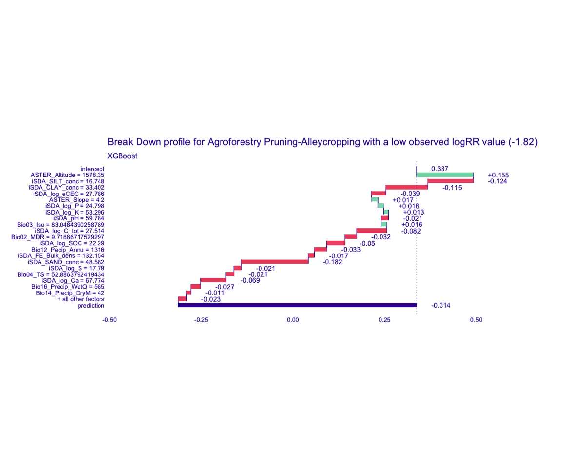
Figure 5: Break-down plot of individial model parts for the XGBoost model low RR
cart model
bd_cart_logRR_low <-
  predict_parts(explainer = explainer_cart_continous,
                new_observation = obs_1,
                type = "break_down")

# SAVING THE BREAK-DOWN PLOT DATA
# saveRDS(bd_cart_logRR_low, here::here("TidyModWflSet_OUTPUT","bd_cart_logRR_low.RDS"))

plot(bd_cart_logRR_low,
     max_features = 20) +
  ggtitle("Break Down profile for Agroforestry Pruning-Alleycropping with a low observed logRR value (-1.82)") +
  theme(panel.grid = element_blank())
Show code
ggdraw() +
  draw_image(here::here("TidyModWflSet_OUTPUT", "bd_cart_logRR_low.png"))

Figure 6: Break-down plot of individial model parts for the cart model low RR
glm model
bd_glm_logRR_low <-
  predict_parts(explainer = explainer_glm_continous,
                new_observation = obs_1,
                type = "break_down")

# SAVING THE BREAK-DOWN PLOT DATA
# saveRDS(bd_glm_logRR_low, here::here("TidyModWflSet_OUTPUT","bd_glm_logRR_low.RDS"))

plot(bd_glm_logRR_low,
     max_features = 20) +
  ggtitle("Break Down profile for Agroforestry Pruning-Alleycropping with a low observed logRR value (-1.82)") +
  theme(panel.grid = element_blank())
Show code
ggdraw() +
  draw_image(here::here("TidyModWflSet_OUTPUT", "bd_cart_logRR_low.png"))
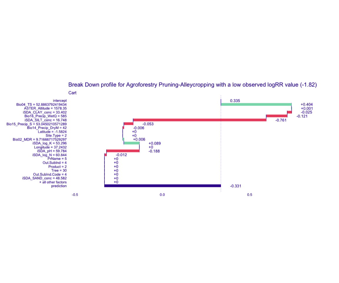
Figure 7: Break-down plot of individial model parts for the glm model low RR
STEP 12e: Visualising break-down of individial model parts for the case of obs_2 (high RR value = 3.04)
Random Forest model
bd_rf_logRR_high <-
  predict_parts(explainer = explainer_rf_continous,
                new_observation = obs_2,
                type = "break_down")

# SAVING THE BREAK-DOWN PLOT DATA
# saveRDS(bd_rf_logRR_high, here::here("TidyModWflSet_OUTPUT","bd_rf_logRR_high.RDS"))

plot(bd_rf_logRR_high,
     max_features = 20) +
  ggtitle("Break Down profile for Agroforestry Pruning-Alleycropping with a high observed logRR value (-1.82)") +
  theme(panel.grid = element_blank())
Show code
ggdraw() +
  draw_image(here::here("TidyModWflSet_OUTPUT", "bd_rf_logRR_high.png"))
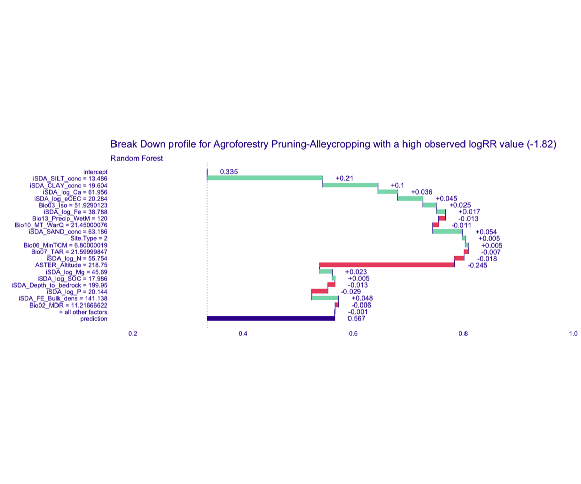
Figure 8: Break-down plot of individial model parts for the Random Forest model high RR
XGBoost model
bd_xgb_logRR_high <-
  predict_parts(explainer = explainer_xgb_continous,
                new_observation = obs_2,
                type = "break_down")

# SAVING THE BREAK-DOWN PLOT DATA
# saveRDS(bd_xgb_logRR_high, here::here("TidyModWflSet_OUTPUT","bd_xgb_logRR_high.RDS"))

plot(bd_xgb_logRR_high,
     max_features = 20) +
  ggtitle("Break Down profile for Agroforestry Pruning-Alleycropping with a high observed logRR value (-1.82)") +
  theme(panel.grid = element_blank())
Show code
ggdraw() +
  draw_image(here::here("TidyModWflSet_OUTPUT", "bd_xgb_logRR_high.png"))
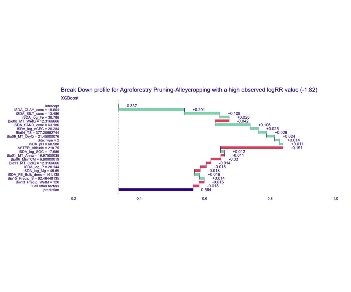
Figure 9: Break-down plot of individial model parts for the XGBoost model high RR
cart model
bd_cart_logRR_high <-
  predict_parts(explainer = explainer_cart_continous,
                new_observation = obs_2,
                type = "break_down")

# SAVING THE BREAK-DOWN PLOT DATA
# saveRDS(bd_cart_logRR_high, here::here("TidyModWflSet_OUTPUT","bd_cart_logRR_high.RDS"))

plot(bd_cart_logRR_high,
     max_features = 20) +
  ggtitle("Break Down profile for Agroforestry Pruning-Alleycropping with a high observed logRR value (-1.82)") +
  theme(panel.grid = element_blank())
Show code
ggdraw() +
  draw_image(here::here("TidyModWflSet_OUTPUT", "bd_cart_logRR_high.png"))
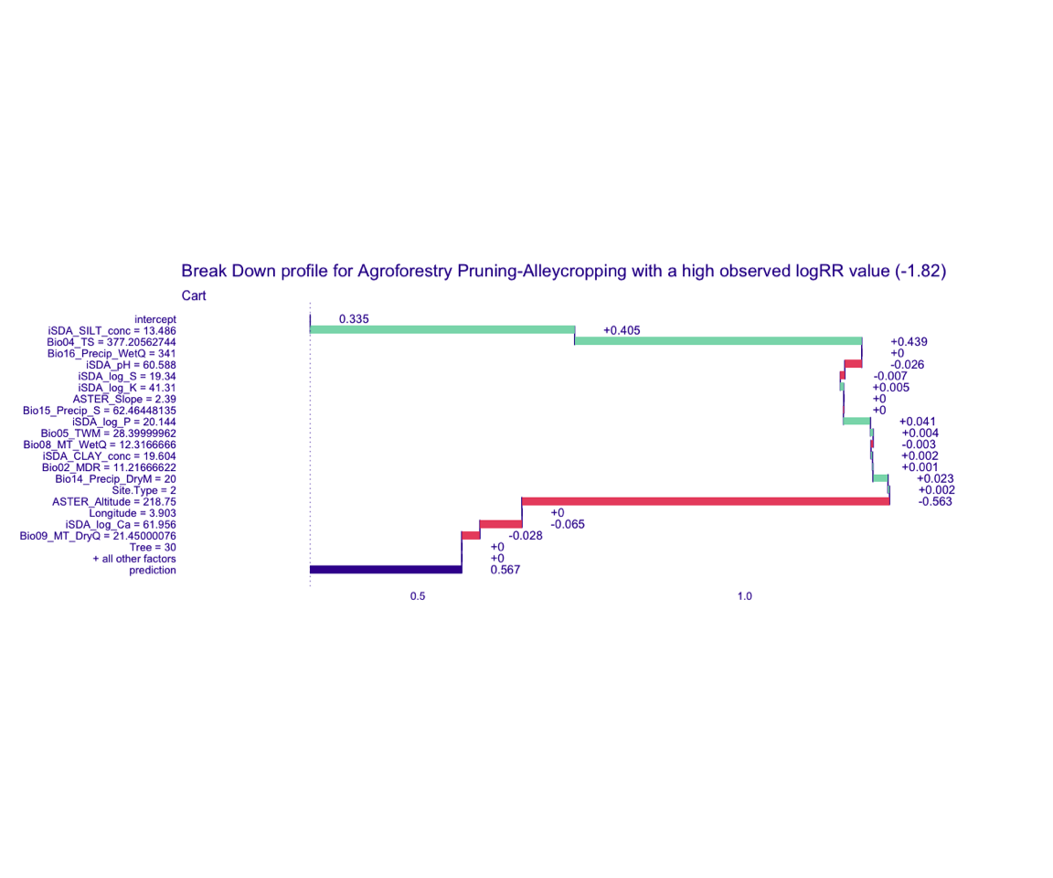
Figure 10: Break-down plot of individial model parts for the cart model high RR
glm model
bd_glm_logRR_high <-
  predict_parts(explainer = explainer_glm_continous,
                new_observation = obs_2,
                type = "break_down")

# SAVING THE BREAK-DOWN PLOT DATA
# saveRDS(bd_glm_logRR_high, here::here("TidyModWflSet_OUTPUT","bd_glm_logRR_high.RDS"))

plot(bd_glm_logRR_high,
     max_features = 20) +
  ggtitle("Break Down profile for Agroforestry Pruning-Alleycropping with a high observed logRR value (-1.82)") +
  theme(panel.grid = element_blank())
Show code
ggdraw() +
  draw_image(here::here("TidyModWflSet_OUTPUT", "bd_glm_logRR_high.png"))
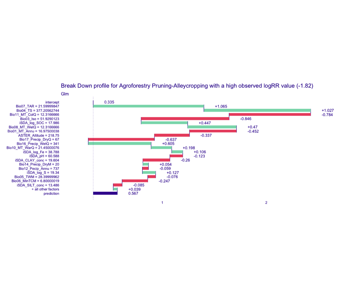
Figure 11: Break-down plot of individial model parts for the glm model high RR
STEP 13: Explaining models and predictions (model agnostics) with SHAP plots
We can use the fact that these break-down explanations change based on order to compute the most important features over all (or many) possible orderings. This is the idea behind Shapley Additive Explanations (Lundberg and Lee 2017), where the average contributions of features are computed under different combinations or “coalitions” of feature orderings. Let’s compute SHAP attributions for our duplex, using B = 20 random orderings. (https://ema.drwhy.ai/breakDown.html).
We could use the default plot method from DALEX by calling plot(shap_obs_1), or we can access the underlying data and create a custom plot.
Creating SHAP plot based on the four different models for the low RR = -1.82
Random Forest
Lets access the underlying data and creating a custom plot with ggplot
The box plots display the distribution of contributions across all the orderings we tried, and the bars display the average attribution for each feature.
Show code
shap_obs_1_rf <- readRDS(here::here("TidyModWflSet_OUTPUT","shap_obs_1_rf.RDS"))

shap_obs_1_rf_plot <-
  shap_obs_1_rf %>%
  group_by(variable) %>%
  mutate(mean_val = mean(contribution)) %>%
  ungroup() %>%
  mutate(variable = fct_reorder(variable, abs(mean_val))) %>%
  ggplot(aes(contribution, variable, fill = mean_val > 0)) +
  geom_col(data = ~distinct(., variable, mean_val),
           aes(mean_val, variable),
           alpha = 0.5) +
  geom_boxplot(width = 0.5) +
  theme(legend.position = "none") +
  labs(y = NULL)


shap_obs_1_rf_plot
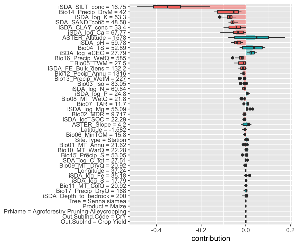
Figure 12: SHAP plot based on the Random Forest model for the low RR observation
We see that for this case the, and in general, the most important environmental features are silt content, precipitation of driest month and the potassium concentration. The shaded areas indicate the global contribution of the variables.
XGBoost model
Show code
shap_obs_1_xgb <- readRDS(here::here("TidyModWflSet_OUTPUT","shap_obs_1_xgb.RDS"))

shap_obs_1_xgb_plot <-
  shap_obs_1_xgb %>%
  group_by(variable) %>%
  mutate(mean_val = mean(contribution)) %>%
  ungroup() %>%
  mutate(variable = fct_reorder(variable, abs(mean_val))) %>%
  ggplot(aes(contribution, variable, fill = mean_val > 0)) +
  geom_col(data = ~distinct(., variable, mean_val),
           aes(mean_val, variable),
           alpha = 0.5) +
  geom_boxplot(width = 0.5) +
  theme(legend.position = "none") +
  labs(y = NULL)


shap_obs_1_xgb_plot
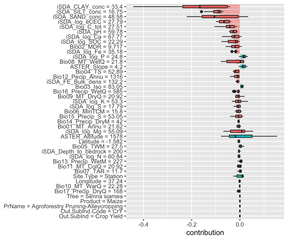
Figure 13: SHAP plot based on the XGB model for the low RR observation
The box plots display the distribution of contributions across all the orderings we tried, and the bars display the average attribution for each feature. We see that for the XGBoost model many of the most important features (e.g. sand, silt, total carbon in the soil) are actually contributing negatively to the predicted response ratios. Both for this case (box plots) and for the general observations (shaded area).
Cart model
Show code
shap_obs_1_cart <- readRDS(here::here("TidyModWflSet_OUTPUT","shap_obs_1_cart.RDS"))

shap_obs_1_cart_plot <-
  shap_obs_1_cart %>%
  group_by(variable) %>%
  mutate(mean_val = mean(contribution)) %>%
  ungroup() %>%
  mutate(variable = fct_reorder(variable, abs(mean_val))) %>%
  ggplot(aes(contribution, variable, fill = mean_val > 0)) +
  geom_col(data = ~distinct(., variable, mean_val),
           aes(mean_val, variable),
           alpha = 0.5) +
  geom_boxplot(width = 0.5) +
  theme(legend.position = "none") +
  labs(y = NULL)


shap_obs_1_cart_plot
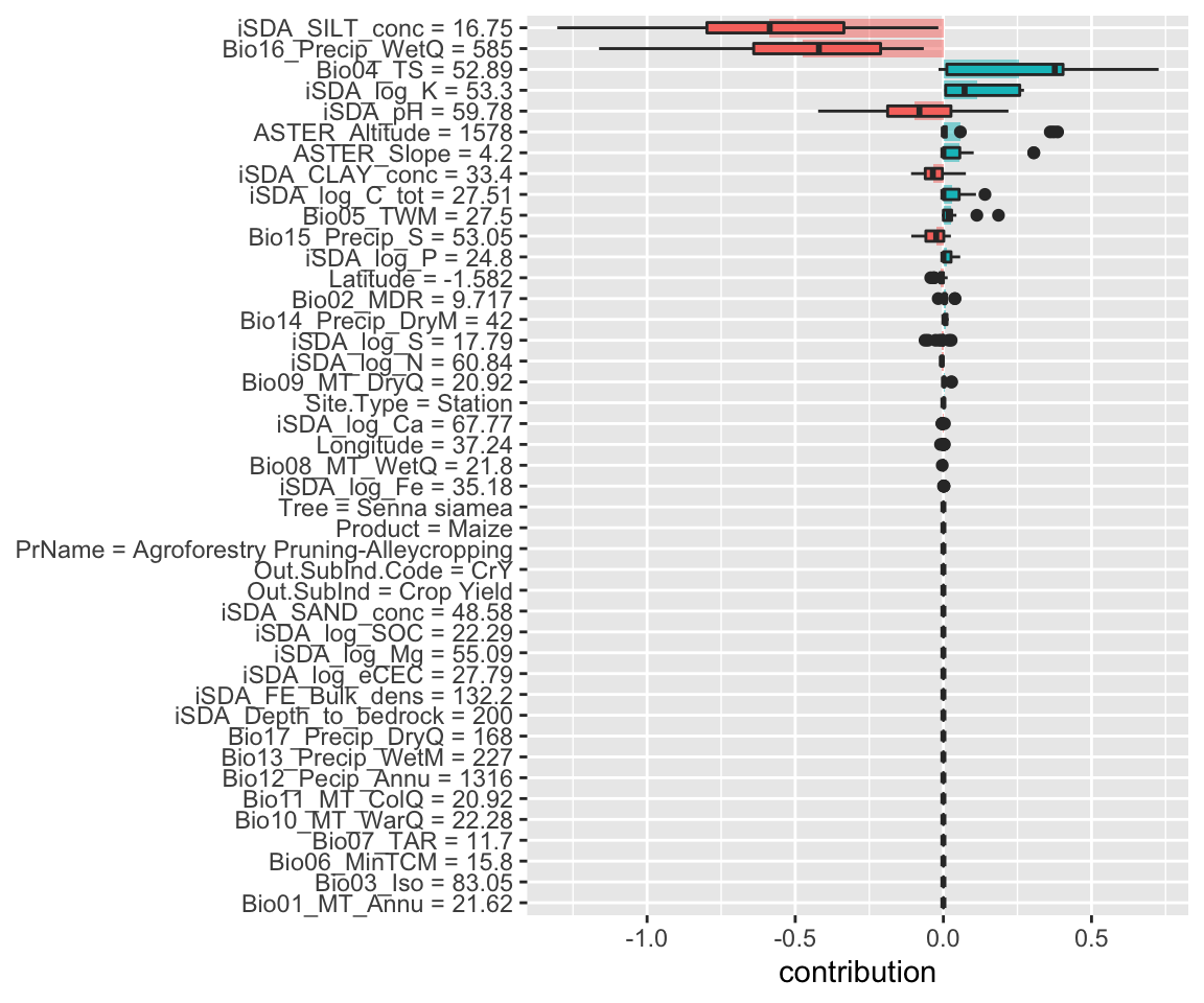
Figure 14: SHAP plot based on the cart model for the low RR observation
Again we see, similar to the Random Forest model, how silt and precipitation negatively contribute to the predicted response ratio values.
glm model
Show code
shap_obs_1_glm <- readRDS(here::here("TidyModWflSet_OUTPUT","shap_obs_1_glm.RDS"))

shap_obs_1_glm_plot <-
  shap_obs_1_glm %>%
  group_by(variable) %>%
  mutate(mean_val = mean(contribution)) %>%
  ungroup() %>%
  mutate(variable = fct_reorder(variable, abs(mean_val))) %>%
  ggplot(aes(contribution, variable, fill = mean_val > 0)) +
  geom_col(data = ~distinct(., variable, mean_val),
           aes(mean_val, variable),
           alpha = 0.5) +
  geom_boxplot(width = 0.5) +
  theme(legend.position = "none") +
  labs(y = NULL)


shap_obs_1_glm_plot
Figure 15: SHAP plot based on the glm model for the low RR observation
With the glm model above we see slightly different patterns emerging compared to the three previous models. Most noticeably is that the precipitation of driest wuarter is now contributing positively to the predicted response ratios.
Lets make similar plots for the other observation with high RR values.
Creating SHAP plot based on the four different models for the high RR = 3.05
Random Forest
Show code
shap_obs_2_rf <- readRDS(here::here("TidyModWflSet_OUTPUT","shap_obs_2_rf.RDS"))

shap_obs_2_rf_plot <-
  shap_obs_2_rf %>%
  group_by(variable) %>%
  mutate(mean_val = mean(contribution)) %>%
  ungroup() %>%
  mutate(variable = fct_reorder(variable, abs(mean_val))) %>%
  ggplot(aes(contribution, variable, fill = mean_val > 0)) +
  geom_col(data = ~distinct(., variable, mean_val),
           aes(mean_val, variable),
           alpha = 0.5) +
  geom_boxplot(width = 0.5) +
  theme(legend.position = "none") +
  labs(y = NULL)


shap_obs_2_rf_plot
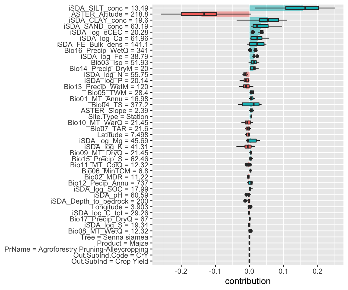
Figure 16: SHAP plot based on the Random Forest model for the high RR observation
We see that the lower silt concentration in this observation (13.49 instead of 16.75) results in a shift from silt being a negative contributor to the response ratios to becoming a positive contributor. This indicates that when soil silt content increase there is a decrease in agroforestry response ratios.
XGBoost model
Show code
shap_obs_2_xgb <- readRDS(here::here("TidyModWflSet_OUTPUT","shap_obs_2_xgb.RDS"))

shap_obs_2_xgb_plot <-
  shap_obs_2_xgb %>%
  group_by(variable) %>%
  mutate(mean_val = mean(contribution)) %>%
  ungroup() %>%
  mutate(variable = fct_reorder(variable, abs(mean_val))) %>%
  ggplot(aes(contribution, variable, fill = mean_val > 0)) +
  geom_col(data = ~distinct(., variable, mean_val),
           aes(mean_val, variable),
           alpha = 0.5) +
  geom_boxplot(width = 0.5) +
  theme(legend.position = "none") +
  labs(y = NULL)


shap_obs_2_xgb_plot
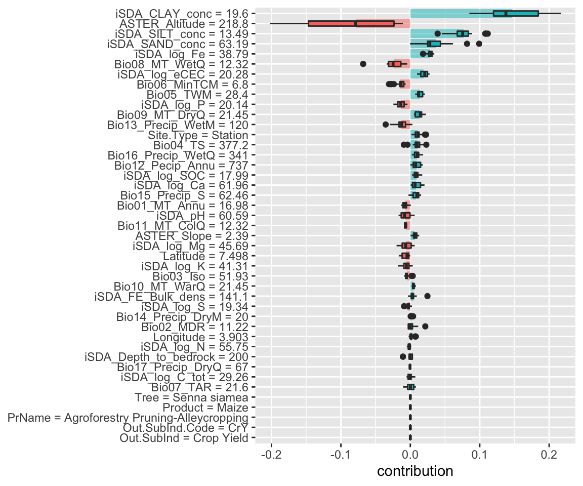
Figure 17: SHAP plot based on the XGB model for the high RR observation
Again the lower clay content and higher sand content contribute positivly to the predicted response ratios
Cart model
Show code
shap_obs_2_cart <- readRDS(here::here("TidyModWflSet_OUTPUT","shap_obs_2_cart.RDS"))

shap_obs_2_cart_plot <-
  shap_obs_2_cart %>%
  group_by(variable) %>%
  mutate(mean_val = mean(contribution)) %>%
  ungroup() %>%
  mutate(variable = fct_reorder(variable, abs(mean_val))) %>%
  ggplot(aes(contribution, variable, fill = mean_val > 0)) +
  geom_col(data = ~distinct(., variable, mean_val),
           aes(mean_val, variable),
           alpha = 0.5) +
  geom_boxplot(width = 0.5) +
  theme(legend.position = "none") +
  labs(y = NULL)


shap_obs_2_cart_plot
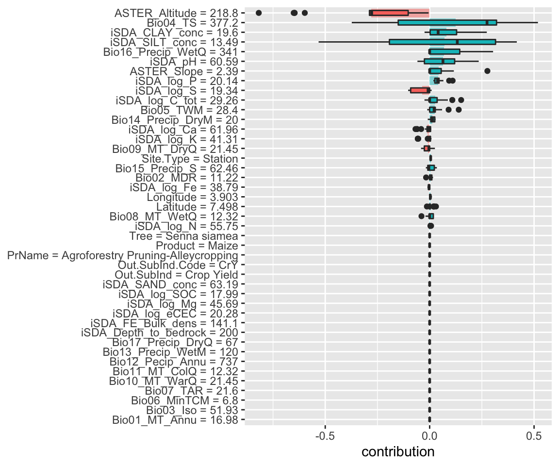
Figure 18: SHAP plot based on the cart model for the high RR observation
Glm model
Show code
shap_obs_2_glm <- readRDS(here::here("TidyModWflSet_OUTPUT","shap_obs_2_glm.RDS"))

shap_obs_2_glm_plot <-
  shap_obs_2_glm %>%
  group_by(variable) %>%
  mutate(mean_val = mean(contribution)) %>%
  ungroup() %>%
  mutate(variable = fct_reorder(variable, abs(mean_val))) %>%
  ggplot(aes(contribution, variable, fill = mean_val > 0)) +
  geom_col(data = ~distinct(., variable, mean_val),
           aes(mean_val, variable),
           alpha = 0.5) +
  geom_boxplot(width = 0.5) +
  theme(legend.position = "none") +
  labs(y = NULL)


shap_obs_2_glm_plot
Figure 19: SHAP plot based on the glm model for the high RR observation
STEP 14: Global model explorations (global model agnostics)
Global model explanations, also called global feature importance or variable importance, help us understand which features are most important in driving the predictions of these two models overall, aggregated over the whole training set. While the previous section addressed what variables or features are most important in predicting sale price for an individual home, global feature importance addresses what variables are most important for a model in aggregate. (read more here: https://www.tmwr.org/explain.html)
Note: One way to compute variable importance is to permute the features (Breiman 2001a). We can permute or shuffle the values of a feature, predict from the model, and then measure how much worse the model fits the data compared to before shuffling.
If shuffling a column causes a large degradation in model performance, it is important; if shuffling a column’s values doesn’t make much difference to how the model performs, it must not be an important variable. This approach can be applied to any kind of model (it is model-agnostic) and the results are straightforward to understand. Using DALEX, we compute this kind of variable importance via the model_parts() function.
Generating vip datasets for each of the four models
Show code
vip_rf <- DALEX::model_parts(explainer_rf, loss_function = loss_root_mean_square)
vip_xgb <- DALEX::model_parts(explainer_xgb, loss_function = loss_root_mean_square)
vip_cart <- DALEX::model_parts(explainer_cart, loss_function = loss_root_mean_square)
vip_glm <- DALEX::model_parts(explainer_glm, loss_function = loss_root_mean_square)

# SAVING THE VIP DATASET
saveRDS(vip_rf, here::here("TidyModWflSet_OUTPUT","vip_rf.RDS"))
saveRDS(vip_xgb, here::here("TidyModWflSet_OUTPUT","vip_xgb.RDS"))
saveRDS(vip_cart, here::here("TidyModWflSet_OUTPUT","vip_cart.RDS"))
saveRDS(vip_glm, here::here("TidyModWflSet_OUTPUT","vip_glm.RDS"))
Again, we could use the default plot method from DALEX by calling e.g. plot(vip_glm) or plot(vip_rf) but the underlying data is available for exploration, analysis, and plotting.
Show code
# plot(vip_rf)
# library(cowplot)

ggdraw() +
  draw_image(here::here("TidyModWflSet_OUTPUT", "vip_rf.png"))
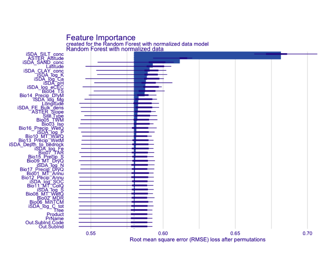
Figure 20: Standadized plot of vip for the RF model
Let’s use the underlying data and create a function that automatically plot our vip model dataset in a ggplot:
ggplot_imp <- function(...) {
  obj <- list(...)
  metric_name <- attr(obj[[1]], "loss_name")
  metric_lab <- paste(metric_name,
                      "after permutations\n(higher indicates more important)")

  full_vip <- bind_rows(obj) %>%
    filter(variable != "_baseline_")

  perm_vals <- full_vip %>%
    filter(variable == "_full_model_") %>%
    group_by(label) %>%
    summarise(dropout_loss = mean(dropout_loss))

  p <- full_vip %>%
    filter(variable != "_full_model_") %>%
    mutate(variable = fct_reorder(variable, dropout_loss)) %>%
    ggplot(aes(dropout_loss, variable))
  if(length(obj) > 1) {
    p <- p +
      facet_wrap(vars(label)) +
      geom_vline(data = perm_vals, aes(xintercept = dropout_loss, color = label),
                 size = 1.2, lty = 2, alpha = 0.7, col = "black") +
      geom_boxplot(aes(color = label, fill = label), alpha = 0.2)
  } else {
    p <- p +
      geom_vline(data = perm_vals, aes(xintercept = dropout_loss),
                 size = 1.2, lty = 2, alpha = 0.7, col = "black") +
      geom_boxplot(fill = "#91CBD765", alpha = 0.4)

  }

  p +
    theme(legend.position = "none") +
    labs(x = metric_lab,
         y = NULL,  fill = NULL,  color = NULL)
}
Using function to plot the vip datasets for each model
Now we can view the vip dataset visually by using the function that was just created. The dashed line in each panel shows the RMSE for the full model, either the linear model or the random forest model. Features further to the right are more important, because permuting them results in higher RMSE. There is quite a lot of interesting information to learn from this plot; for example, neighborhood is quite important in the linear model with interactions/splines but the second least important feature for the random forest model.
VIP for the tree-based models RF and XGBShow code
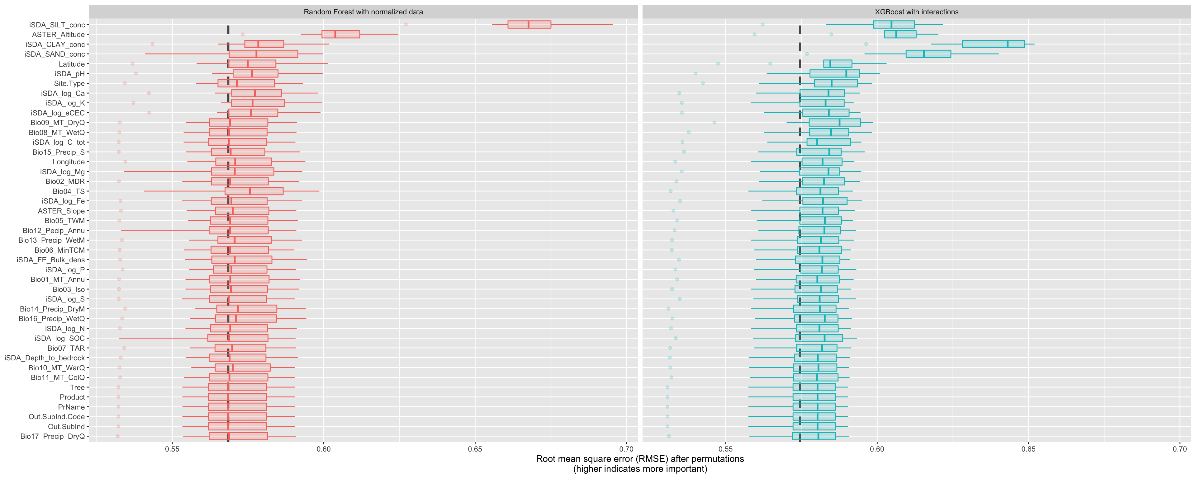
Figure 21: Costumn plot of the vip using the special ggplot function for the tree-based models
Show code
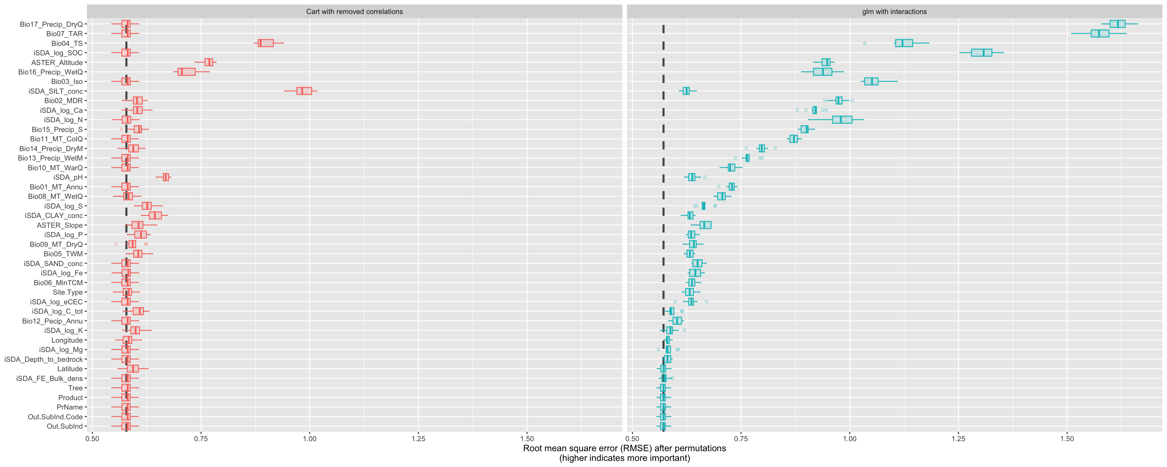
Figure 22: Costumn plot of the vip using the special ggplot function for the cart and glm models
The differences are quite substantial!
STEP 15: Model exploration and agnosticcs from partial dependencce plots
BUILDING GLOBAL EXPLANATIONS FROM LOCAL EXPLANATIONS. So far we have focused on local model explanations for a single observation (via Shapley additive explanations) and global model explanations for a data set as a whole (via permuting features). It is also possible to build global model explanations up by aggregating local model explanations, as with partial dependence profiles.
Note: Partial dependence profiles show how the expected value of a model prediction, like the response ratio of agroforestry, changes as a function of a particular feature, like the precipitation of driest quarter or soil sand content.
One way to build such a profile is by aggregating or averaging profiles for individual observations. A profile showing how an individual observation’s prediction changes as a function of a given feature is called an ICE (individual conditional expectation) profile or a CP (ceteris paribus) profile. We can compute such individual profiles (for 500 of the observations in our training set) and then aggregate them using the DALEX function model_profile(). pdp = partial dependency plots
Let’s create another function for plotting the underlying data in this object:
ggplot_pdp <- function(obj, x) {

  p <-
    as_tibble(obj$agr_profiles) %>%
    mutate(`_label_` = stringr::str_remove(`_label_`, "^[^_]*_")) %>%
    ggplot(aes(`_x_`, `_yhat_`)) +
    geom_line(data = as_tibble(obj$cp_profiles),
              aes(x = {{ x }}, group = `_ids_`),
              size = 0.5, alpha = 0.05, color = "gray50")

  num_colors <- n_distinct(obj$agr_profiles$`_label_`)

  if (num_colors > 1) {
    p <- p + geom_line(aes(color = `_label_`), size = 1.2, alpha = 0.8)
  } else {
    p <- p + geom_line(color = "midnightblue", size = 1.2, alpha = 0.8)
  }

  p
}
Show code
# LOADING/READING THE EXPLAINERS
explainer_rf <- readRDS(here::here("TidyModWflSet_OUTPUT","explainer_rf.RDS"))
# explainer_xgb <- readRDS(here::here("TidyModWflSet_OUTPUT","explainer_rf.RDS"))
# explainer_rf <- readRDS(here::here("TidyModWflSet_OUTPUT","explainer_rf.RDS"))
# explainer_rf <- readRDS(here::here("TidyModWflSet_OUTPUT","explainer_rf.RDS"))

# Random Forest model
# -----------------------------------------------------------------------------------
# Silt content
pdp_iSDA_SILT <- model_profile(explainer_rf,
                               N = 500,
                               variables = "iSDA_SILT_conc")

# Sand content
pdp_iSDA_SAND <- model_profile(explainer_rf,
                               N = 500,
                               variables = "iSDA_SAND_conc")

# Mean diurnal temperature range
pdp_Bio02_MDR <- model_profile(explainer_rf,
                               N = 500,
                               variables = "Bio02_MDR")

# Precipitation of driest quarter
pdp_Bio09_MT_DryQ <- model_profile(explainer_rf,
                               N = 500,
                               variables = "Bio17_Precip_DryQ")

# Temperature Sum
pdp_Bio04_TS <- model_profile(explainer_rf,
                              N = 500,
                              variables = "Bio04_TS")

#GROUPINGS

# Sand content with grouping of Site Type (research station / farm)
pdp_iSDA_SAND_conc_sitetype <- model_profile(explainer_rf,
                              N = 500,
                              variables = "iSDA_SAND_conc",
                              groups = "Site.Type")

# Sand content with grouping of Tree speies (what species of tree)
pdp_iSDA_SAND_conc_tree <- model_profile(explainer_rf,
                              N = 500,
                              variables = "iSDA_SAND_conc",
                              groups = "Tree") #%>%
  #dplyr::filter(Tree == "Faidherbia albida" |
  #                Tree == "Cassia spectabilis")
Show code
ggplot_pdp(pdp_iSDA_SILT, iSDA_SILT_conc)  +
  labs(x = "Soil SILT content",
       y = "Predicted response ratio (log scale)",
       color = NULL) +
  ggtitle("Partial dependence plot based on the Random Forest model, feature: Silt content")

Figure 23: Partial dependence plot for silt content
Show code
ggplot_pdp(pdp_iSDA_SAND, iSDA_SAND_conc)  +
  labs(x = "Soil SAND content",
       y = "Predicted response ratio (log scale)",
       color = NULL)  +
  ggtitle("Partial dependence plot based on the Random Forest model, feature: Sand content")
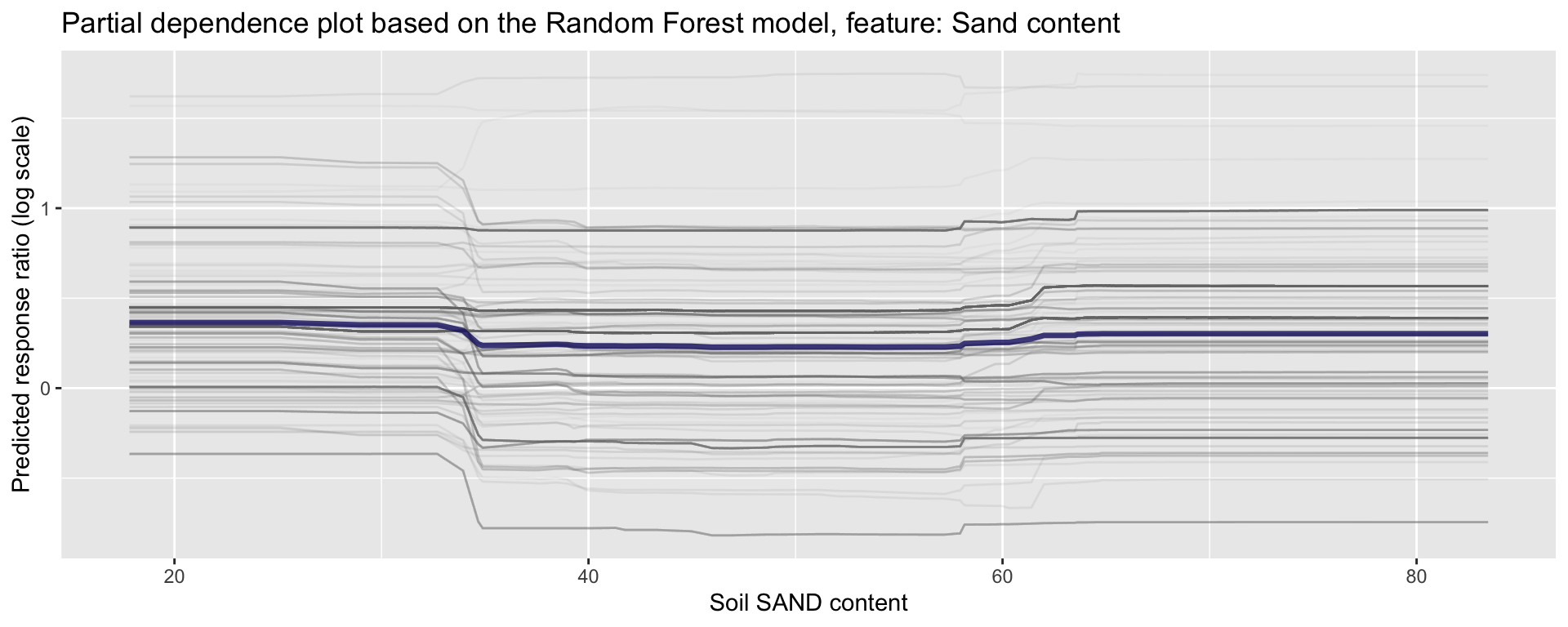
Figure 24: Partial dependence plot for sand content
Show code
ggplot_pdp(pdp_Bio02_MDR, Bio02_MDR)  +
  labs(x = "Mean Diurnal Temperature Range",
       y = "Predicted response ratio (log scale)",
       color = NULL)  +
  ggtitle("Partial dependence plot based on the Random Forest model, feature: Mean Diurnal Temperature Range")
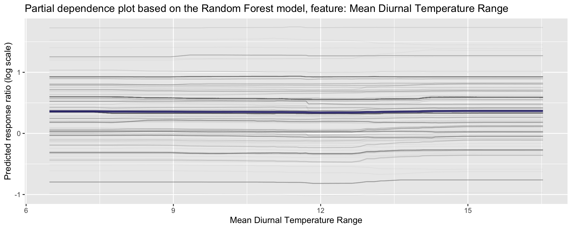
Figure 25: Partial dependence plot for Mean Diurnal Temperature Range
Show code
ggplot_pdp(pdp_Bio09_MT_DryQ, Bio17_Precip_DryQ)  +
  labs(x = "Precipitation of Driest Quarter",
       y = "Predicted response ratio (log scale)",
       color = NULL)  +
  ggtitle("Partial dependence plot based on the Random Forest model, feature: Precipitation of Driest Quarter")
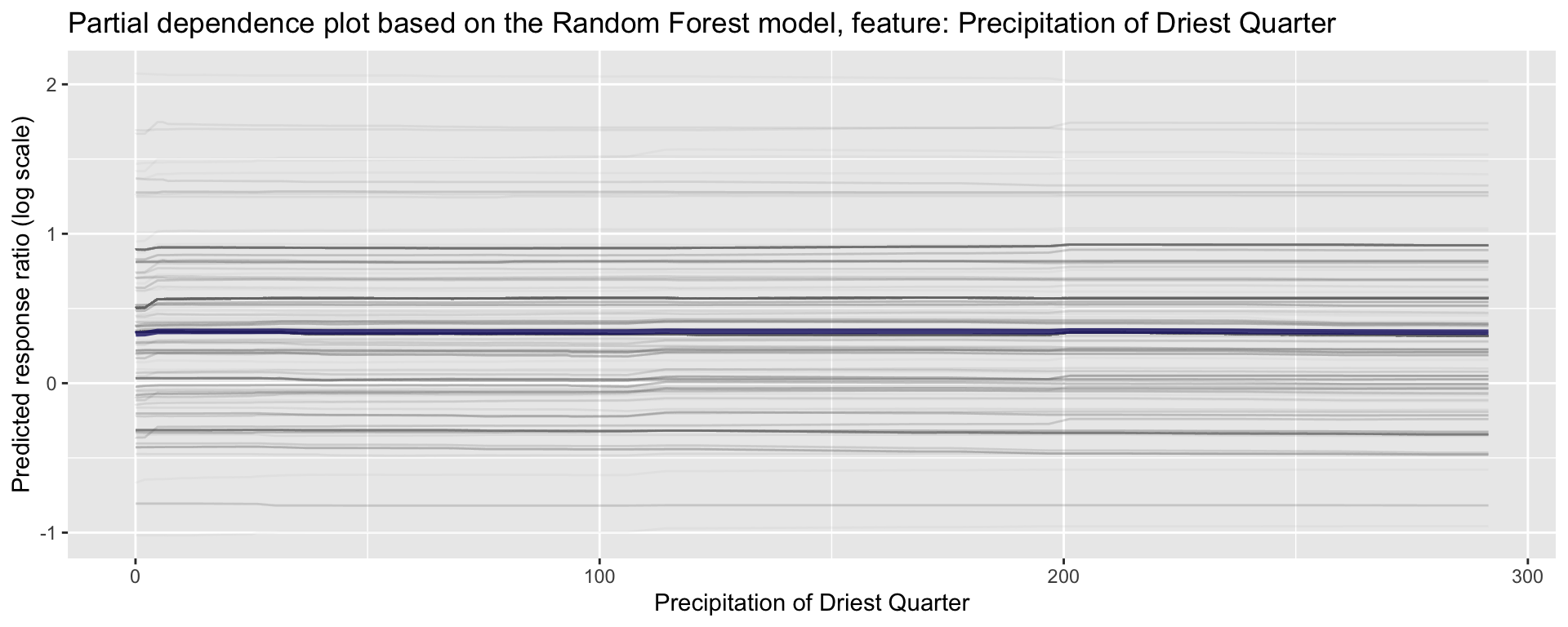
Figure 26: Partial dependence plot for Precipitation of Driest Quarter
Show code
ggplot_pdp(pdp_Bio04_TS, Bio04_TS)  +
  labs(x = "Temperature Sum",
       y = "Predicted response ratio (log scale)",
       color = NULL)  +
  ggtitle("Partial dependence plot based on the Random Forest model, feature: Temperature Sum")
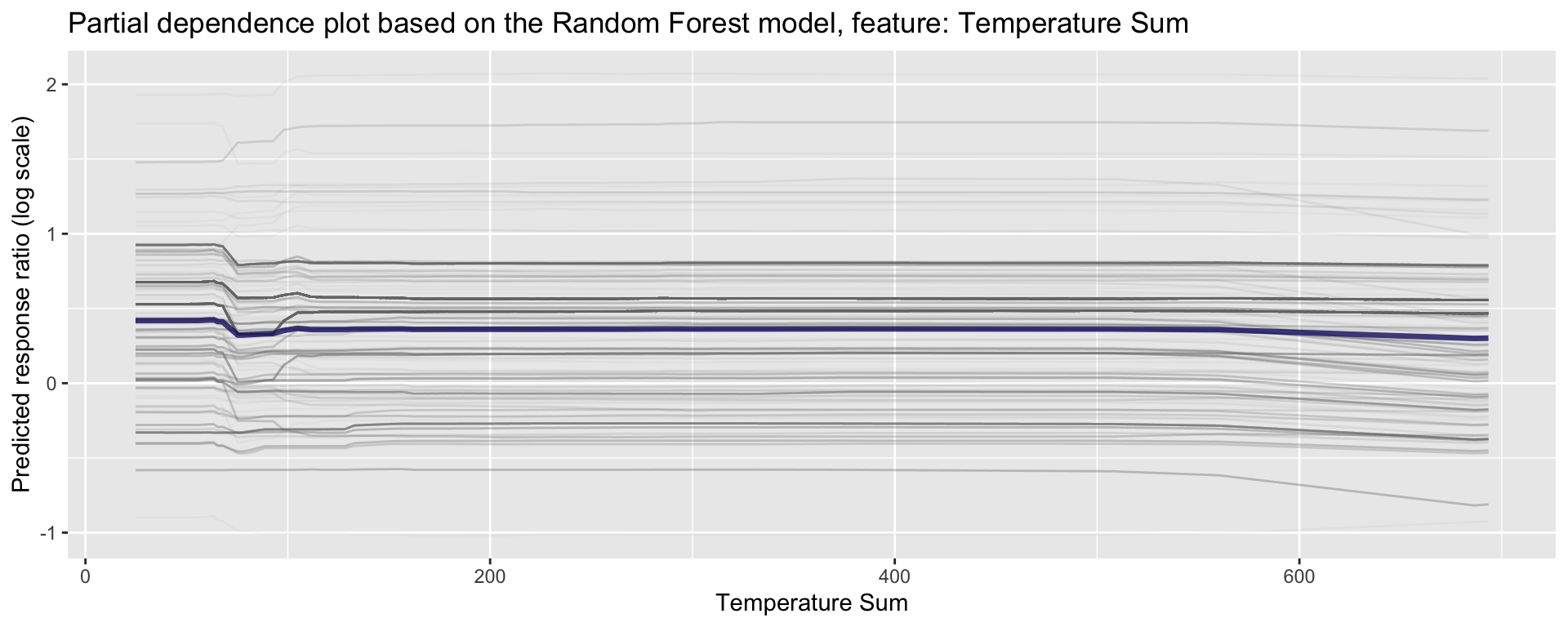
Figure 27: Partial dependence plot for Temperature Sumr
Partial dependence profiles can be computed for any other feature in the model, and also for groups in the data. Let’s try making a partial dependence plot of the groups of Site Type. In this way we can identify potential differences between response on researcch stations and/or farms. We will use the environmental predictor feature “Sand content”:
Partial dependence plot on Sand content with grouping of Tree specciesShow code
ggplot_pdp(pdp_iSDA_SAND_conc_sitetype, iSDA_SAND_conc)  +
  labs(x = "Sand content",
       y = "Predicted response ratio (log scale)",
       color = NULL)  +
  ggtitle("Partial dependence plot based on the Random Forest model, feature: Sand content with grouping of Site Type")
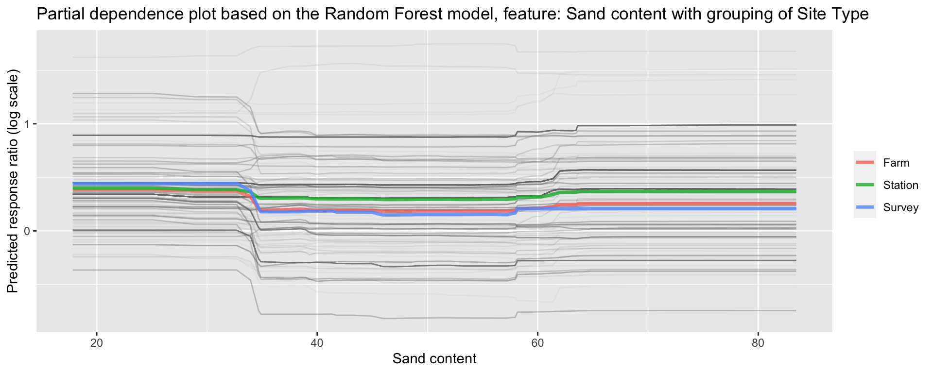
Figure 28: Partial dependence plot for Grouping of Site Type on Sand content
We see there is a slight difference with experiments conducted at stations and survey data having generally higher predicted response ratios..? That is interesting!
Let’s see for tree species:
Partial dependence plot on Sand content with grouping of Tree speciesShow code
ggplot_pdp(pdp_iSDA_SAND_conc_tree, iSDA_SAND_conc)  +
  labs(x = "Soil SAND content",
       y = "Predicted response ratio (log scale)",
       color = NULL)  +
  ggtitle("Partial dependence plot based on the Random Forest model, feature: Sand content with grouping of Tree species") +
  theme(legend.position="bottom")
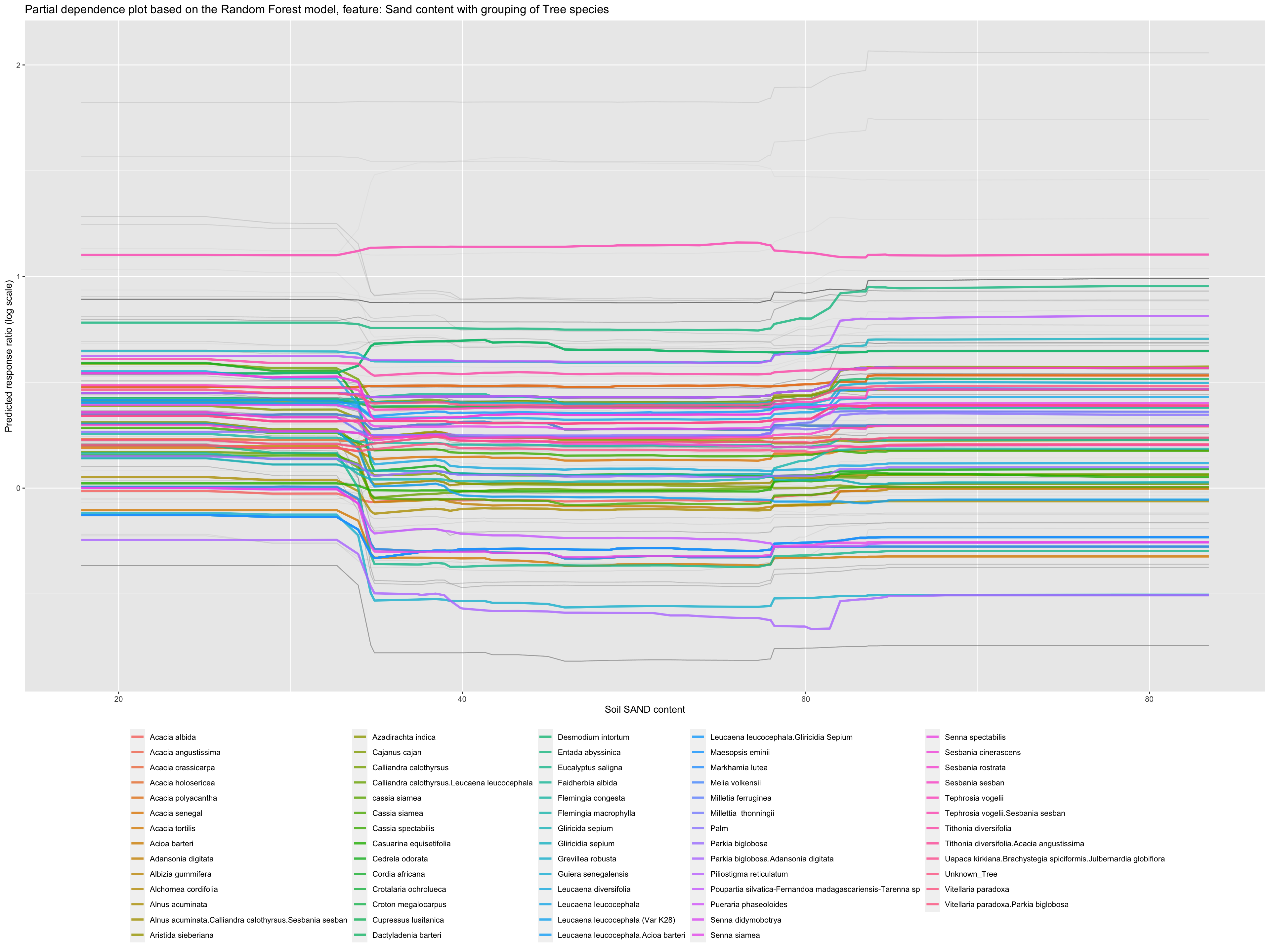
Figure 29: Partial dependence plot for Sand content with grouping of Tree species
STEP 16: Global model partial dependencce plots
We can show how each model predicts depending on a selected feature using the “type =”partial"" argument and then add all our models.
Show code
# LOADING/READING EXPLAINERS
explainer_rf_continous <- readRDS(here::here("TidyModWflSet_OUTPUT","explainer_rf_continous.RDS"))
explainer_xgb_continous <- readRDS(here::here("TidyModWflSet_OUTPUT","explainer_xgb_continous.RDS"))
explainer_cart_continous <- readRDS(here::here("TidyModWflSet_OUTPUT","explainer_cart_continous.RDS"))
explainer_glm_continous <- readRDS(here::here("TidyModWflSet_OUTPUT","explainer_glm_continous.RDS"))

pdp_rf_grade <- model_profile(explainer_rf_continous, variable = "iSDA_SAND_conc", type = "partial")
pdp_xgb_grade <- model_profile(explainer_xgb_continous, variable = "iSDA_SAND_conc", type = "partial")
pdp_cart_grade <- model_profile(explainer_cart_continous, variable = "iSDA_SAND_conc", type = "partial")
pdp_glm_grade <- model_profile(explainer_glm_continous, variable = "iSDA_SAND_conc", type = "partial")
Show code
plot(pdp_rf_grade, pdp_xgb_grade, pdp_cart_grade, pdp_glm_grade)
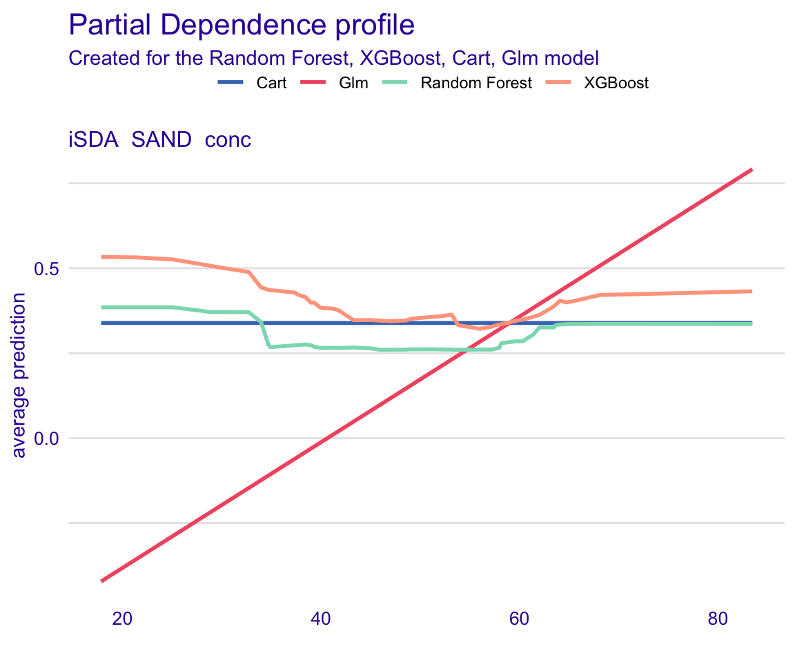
Figure 30: Global model partial dependencce plots for feature; Sand content
STEP 17: Global model residual evaluation
Show code
rf_modperf <- DALEX::model_performance(explainer_rf_continous)
xgb_modperf <- DALEX::model_performance(explainer_xgb_continous)
cart_modperf <- DALEX::model_performance(explainer_cart_continous)
glm_modperf <- DALEX::model_performance(explainer_glm_continous)
Show code
plot(rf_modperf, xgb_modperf, cart_modperf, glm_modperf)
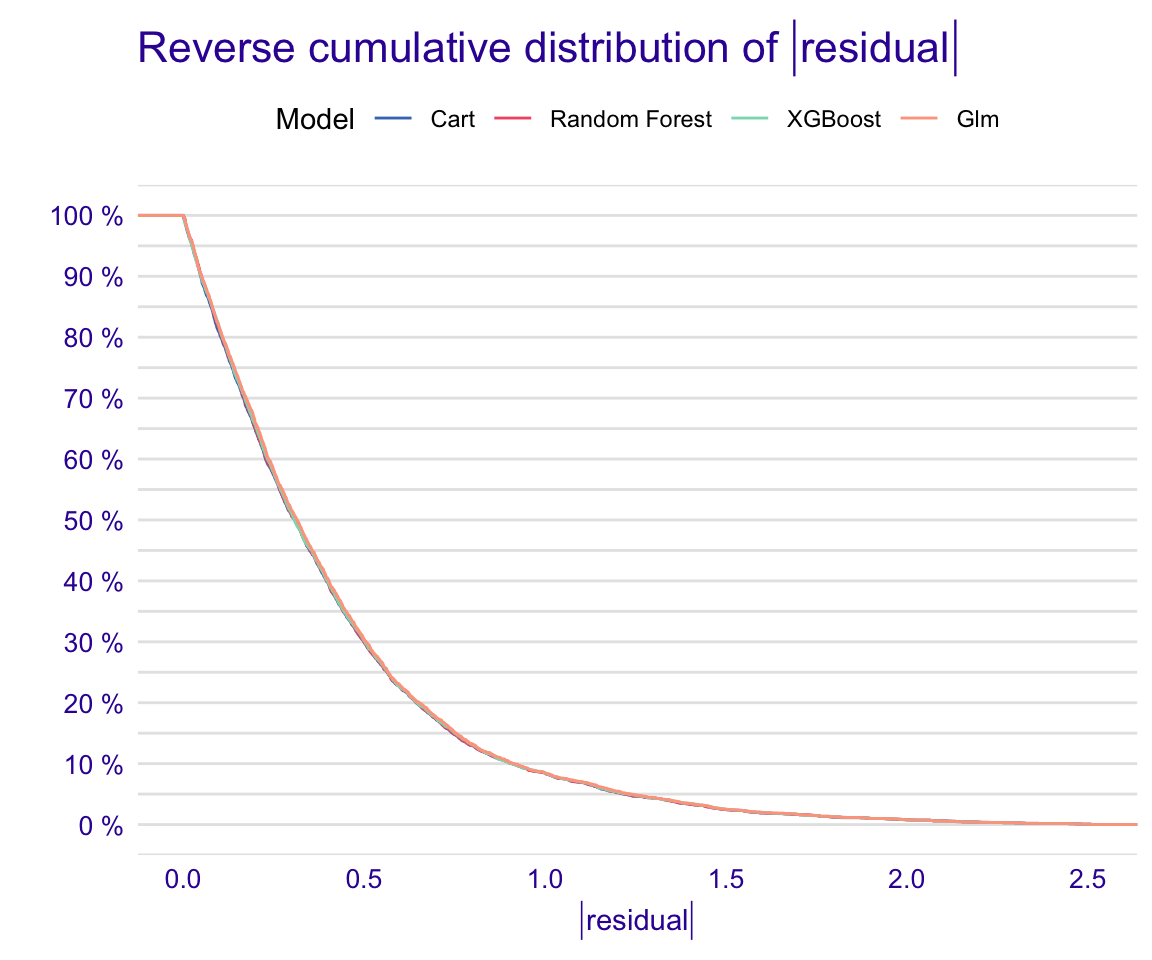
Figure 31: Global model residual evaluation: Reverse cumulative of the absolute residual plot
From the reverse cumulative of the absolute residual plot, we can see that the models are extremly similar! It shows a higher number of large residuals in the left hand side compared to right for all the models.
Show code
plot(rf_modperf, xgb_modperf, cart_modperf, glm_modperf, geom = "boxplot")
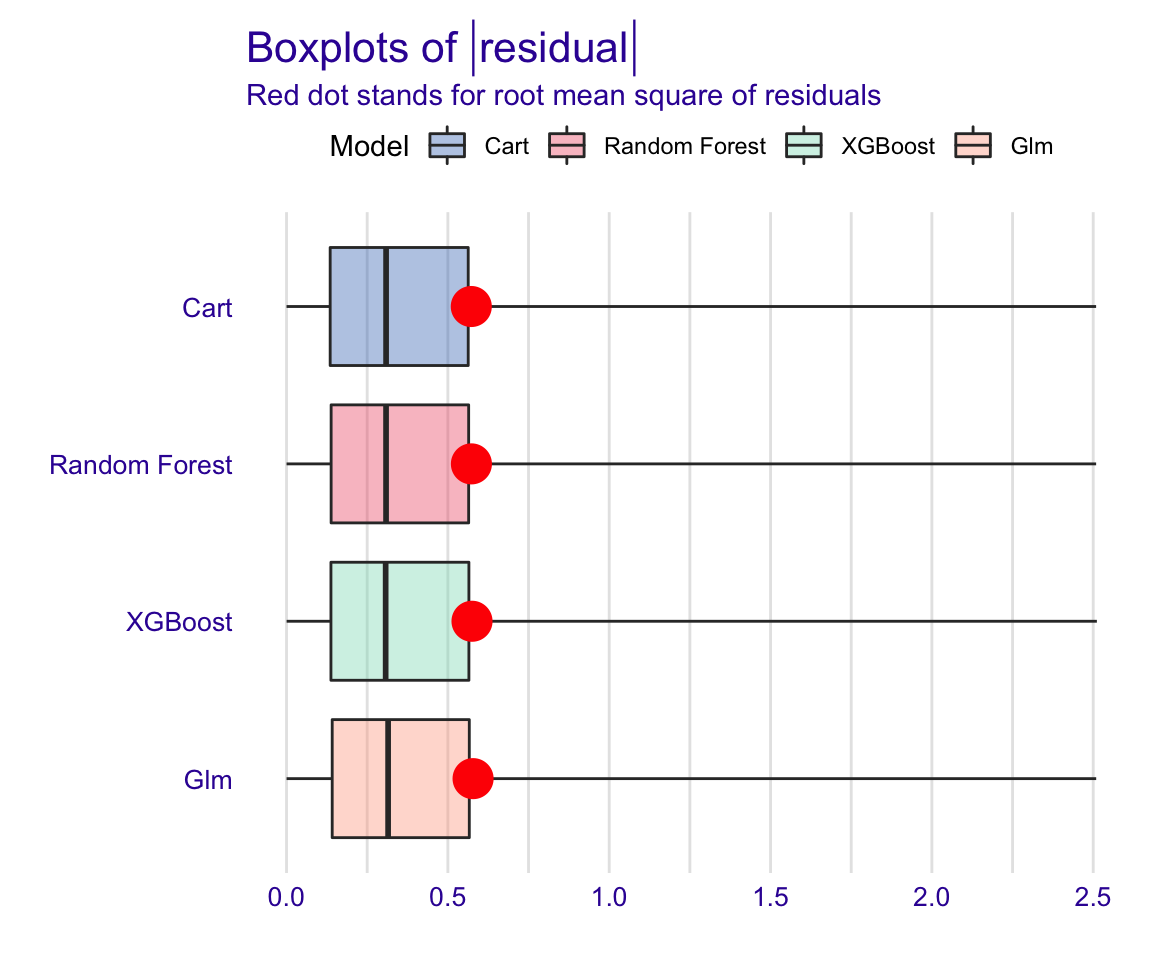
Figure 32: Global model residual evaluation: Boxplot of mean residual vavlues
The boxplot figure above shows that all models have very similar median absolute residual values. We can also plot the distribution of residuals with histograms by using geom=“histogram” and the precision recall curve by using geom=“prc.” Let’s use the geom=“histogram” to vvisualise the distribution of residuals of the models:
Show code
plot(rf_modperf, xgb_modperf, cart_modperf, glm_modperf, geom = "histogram")
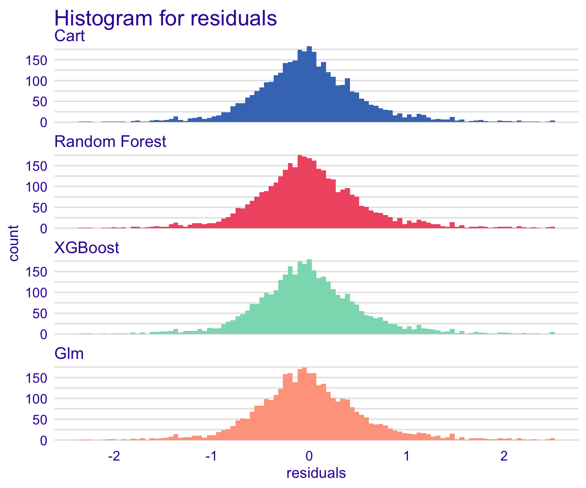
Figure 33: Global model residual evaluation: Residual distribution histogram
The residuals of the models follow to a great deal the normal distribution, which is a good sign!
STEP 18: Global and local model explorotive analysis (agnostics) using Ceteris Paribus Profiles (CPP)
In the previous section, we have discussed the partial dependence plots. The Ceteris Paribus Profiles (CPP) is the single observation level version of the PDP plots. To create this plot, we can use predict_profile() function in the DALEX package. In the following example, we select two predictors for the same observation (i.e., student 1) and create a CPP plot for the RF model. In the plot, blue dots represent the original values for the selected observation.
Generating new observation for the CPP plot
Show code
new_obs_1 <- data.frame(PrName = factor("Agroforestry Pruning-Alleycropping", levels = c("Parklands", "Agroforestry Pruning-Organic Fertilizer",
                                                                                          "Agroforestry Pruning", "Agroforestry Pruning-Inorganic Fertilizer",
                                                                                          "Agroforestry Pruning-Alleycropping", "Alleycropping",
                                                                                          "Agroforestry Pruning-Alleycropping-Inorganic Fertilizer",
                                                                                          "Alleycropping-Inorganic Fertilizer", "Agroforestry Pruning-Alleycropping-Organic Fertilizer",
                                                                                          "Agroforestry Pruning-Alleycropping-Reduced Tillage", "Agroforestry Pruning-Parklands",
                                                                                          "Agroforestry Pruning-Boundary Planting",
                                                                                          "Agroforestry Pruning-Boundary Planting-Inorganic Fertilizer",
                                                                                          "Agroforestry Fallow-Agroforestry Pruning",
                                                                                          "Agroforestry Fallow-Agroforestry Pruning-Alleycropping",
                                                                                          "Agroforestry Pruning-Alleycropping-Intercropping",
                                                                                          "Agroforestry Pruning-Green Manure", "Agroforestry Pruning-Green Manure-Inorganic Fertilizer",
                                                                                          "Agroforestry Fallow",  "Agroforestry Fallow-Water Harvesting",
                                                                                          "Agroforestry Fallow-Agroforestry Pruning-Reduced Tillage", "Agroforestry Pruning-Intercropping",
                                                                                          "Other Agroforestry", "Mulch-Other Agroforestry-Reduced Tillage",
                                                                                          "Agroforestry Pruning-Reduced Tillage-Water Harvesting")),
                        Out.SubInd = factor("Crop Yield", levels = c("Biomass Yield", "Soil Organic Carbon", "Soil Nitrogen", "Crop Yield", "Carbon Dioxide Emissions", "Gross Return",
                                                                      "Marginal Rate of Return", "Beneficial Organisms", "Nitrogen Use Efficiency (ARE AGB)", "Cation Exchange Capacity",
                                                                      "Phosphorus Use Efficiency (ARE AGB)", "Potassium Use Efficiency (ARE AGB)", "Soil Organic Carbon (Change)",
                                                                      "Water Use Efficiency", "Soil Moisture", "Labour Person Hours", "Labour Cost", "Variable Cost", "Net Return",
                                                                      "Benefit Cost Ratio (NRTC)", "Return to Labour", "Gross Margin", "Benefit Cost Ratio (GRVC)", "Net Present Value",
                                                                      "Biodiversity", "Phosphorus Agronomic Efficiency", "Soil Organic Matter", "Nitrogen Factor Productivity", "Water Use",
                                                                      "Infiltration Rate", "Runoff", "Erosion", "Soil Total Nitrogen", "Soil Carbon Stocks", "Soil Available Nitrogen",
                                                                      "Nitrous Oxide Emissions", "Methane Emissions", "CO2 Equivalent Emissions", "Benefit Cost Ratio (GRTC)", "Soil NH4",
                                                                      "Soil NO3", "Land Equivalent Ratio")),
                        Product = factor("Maize", levels = c("Pearl Millet", "Maize", "Wheat", "Sorghum", "Tomato (Total Yield)", "Common Bean", "Okra", "Spinach", "Sunflower (Seed)",
                                                              "Rice", "Sunflower (Oil)", "Sesame Seed", "Eggplant", "Barley", "Finger Millet", "Soybean")),
                        Tree = factor("Senna siamea", levels = c("Faidherbia albida", "Aristida sieberiana", "Guiera senegalensis", "Calliandra calothyrsus", "Sesbania sesban",
                                                                  "Leucaena leucocephala", "Leucaena pallida", "Acacia albida", "Albizia gummifera", "Cordia africana",
                                                                  "Croton macrostachyus", "Milletia ferruginea", "Gliricidia sepium", "Unknown_Tree", "Alnus acuminata",
                                                                  "Alnus acuminata.Calliandra calothyrsus.Sesbania sesban", "Calliandra calothyrsus.Leucaena leucocephala",
                                                                  "Crotalaria juncea", "Cupressus lusitanica", "Casuarina equisetifolia", "Markhamia lutea", "Melia azedarach",
                                                                  "Cordia abyssinica", "Maesopsis eminii", "Senna spectabilis", "Tithonia diversifolia", "Acacia tumida",
                                                                  "Eucalyptus saligna", "Flemingia macrophylla", "Senna siamea", "Leucaena leucocephala.Gliricidia Sepium",
                                                                  "Croton megalocarpus", "Melia volkensii", "Croton megalocarpus.Melia volkensii.Senna spectabilis.Gliricidia sepium",
                                                                  "Pinus patula", "Acacia saligna", "Crotalaria grahamiana", "Grevillea robusta", "Paulownia fortunei",
                                                                  "Entada abyssinica", "Dactyladenia barteri", "Gliricidia", "Flemingia", "Cinnamomum cassia","Flemingia congesta",
                                                                  "Cassia siamea", "cassia siamea", "Leucaena leucocephala.Acioa barteri", "Acioa barteri", "Azadirachta indica",
                                                                  "Parkia biglobosa", "Millettia  thonningii", "Pterocarpus santalinoides", "Acacia angustissima",
                                                                  "Tithonia diversifolia.Acacia angustissima", "Tithonia diversifolia.Calliandra calothyrsus",
                                                                  "Tithonia diversifolia.Flemingia macrophylla", "Elaeis guineensis", "Leucaena leucocephala (Var K28)",
                                                                  "Cajanus cajan", "Leucaena.Azadirachta indica.Parkia biglobosa",
                                                                  "Senna siamea.Leucaena leucocephala.Azadirachta indica", "Vitellaria paradoxa.Parkia biglobosa", "Vitellaria paradoxa",
                                                                  "Parkia biglobosa.Vitellaria paradoxa", "Parkia biglobosa.Adansonia digitata", "Stylosanthes hamata",
                                                                  "Adansonia digitata", "Albizia lebbeck", "Acacia holosericea", "Palm", "Acacia senegal", "Acacia crassicarpa",
                                                                  "Acacia mangium", "Acacia polyacantha", "Leucaena diversifolia", "Tephrosia vogelii.Sesbania sesban",
                                                                  "Alchornea cordifolia", "Uapaca kirkiana.Brachystegia spiciformis.Julbernardia globiflora", "Uapaca kirkiana",
                                                                  "Sesbania rostrata", "Cassia spectabilis", "Grevillea robusta.Cajanus cajan", "Tephrosia vogelii", "Sesbania cinerascens",
                                                                  "Senna didymobotrya", "Senna occidentalis", "Eucalyptus camaldulensis", "Pueraria phaseoloides", "Acacia leptocarpa",
                                                                  "Gliricida sepium", "Flemingia macrophylla.Gliricidia sepium", "Cedrela serrata", "Acrocarpus fraxinifolius",
                                                                  "Cedrela odorata", "Erythrina poeppigiana", "Albizia chinensis", "Piliostigma reticulatum",
                                                                  "Poupartia silvatica-Fernandoa madagascariensis-Tarenna sp", "Acacia tortilis", "Crotalaria ochrolueca",
                                                                  "Desmodium intortum", "Bauhinia reticulata", "Bauhinia reticulata-Guiera senegalensis", "Acacia sp")),
                        Out.SubInd.Code = factor("CrY", levels = c("BiY", "SOC", "SN", "CrY", "CO2", "GR", "MRR", "BO", "NUE-Aag", "CEC", "PUE-Aag", "KUE-Aag", "SOCh", "WUE", "SM",
                                                                    "La-ph", "LC", "VC", "NR", "BCR-NRTC", "RtL", "GM", "BCR-GRVC", "NOV", "Bd", "PAEp", "SOM", "NTFP", "WU", "In",
                                                                    "Ru", "Er", "STN", "SCS", "SAN", "NOx", "CH4", "CO2eq", "BCR-GRTC", "SNH4", "SNO3", "LER")),
                        Site.Type = factor("Station", levels = c("Farm", "Station", "Survey")),
                        Latitude = -1.5824,
                        Longitude = 37.2432,

                        Bio01_MT_Annu = 21.61667,
                        Bio02_MDR = 9.716667,
                        Bio03_Iso = 83.04844,
                        Bio04_TS = 52.88638,
                        Bio05_TWM = 27.5,
                        Bio06_MinTCM = 15.8,
                        Bio07_TAR = 11.7,
                        Bio08_MT_WetQ = 21.8,
                        Bio09_MT_DryQ = 20.91667,
                        Bio10_MT_WarQ = 22.28333,
                        Bio11_MT_ColQ = 20.91667,
                        Bio12_Pecip_Annu = 1316,
                        Bio13_Precip_WetM = 227,
                        Bio14_Precip_DryM = 42,
                        Bio15_Precip_S = 53.04502,
                        Bio16_Precip_WetQ = 585,
                        Bio17_Precip_DryQ = 168,
                        iSDA_Depth_to_bedrock = 199.99,
                        iSDA_SAND_conc = 48.582,
                        iSDA_CLAY_conc = 33.402,
                        iSDA_SILT_conc = 16.748,
                        iSDA_log_C_tot = 27.514  ,
                        iSDA_FE_Bulk_dens = 132.154,
                        iSDA_log_Ca = 67.774,
                        iSDA_log_eCEC = 27.786,
                        iSDA_log_Fe = 35.182,
                        iSDA_log_K = 53.296,
                        iSDA_log_Mg = 55.09,
                        iSDA_log_N = 60.844,
                        iSDA_log_SOC = 22.29,
                        iSDA_log_P = 24.798,
                        iSDA_log_S = 17.79,
                        iSDA_pH = 59.784,
                        ASTER_Altitude = 1578.35,
                        ASTER_Slope = 4.2)
Creating dataset for the CPP for all the four models (with a relatively low RR observation)
- logRR = -0.3305098
# Random Forest  ---------------------------------------------------------

cpp_newObs_1_rf <- DALEX::predict_profile(explainer_rf_continous, new_obs_1)

# XGBoost  ---------------------------------------------------------

cpp_newObs_1_xgb <- DALEX::predict_profile(explainer_xgb_continous, new_obs_1)

# Cart model  ---------------------------------------------------------

cpp_newObs_1_caret <- DALEX::predict_profile(explainer_cart_continous, new_obs_1)

# Glm model ---------------------------------------------------------

cpp_newObs_1_glm <- DALEX::predict_profile(explainer_glm_continous, new_obs_1)


# SAVING THE CPP DATA
saveRDS(cpp_newObs_1_rf, here::here("TidyModWflSet_OUTPUT","cpp_newObs_1_rf.RDS"))
saveRDS(cpp_newObs_1_xgb, here::here("TidyModWflSet_OUTPUT","cpp_newObs_1_xgb.RDS"))
saveRDS(cpp_newObs_1_caret, here::here("TidyModWflSet_OUTPUT","cpp_newObs_1_caret.RDS"))
saveRDS(cpp_newObs_1_glm, here::here("TidyModWflSet_OUTPUT","cpp_newObs_1_glm.RDS"))
Visualising the CPP for the Random Forest model for selected environmental predictor features
SOIL: CPP for RF with clay content, phosphorus concentration and pHShow code
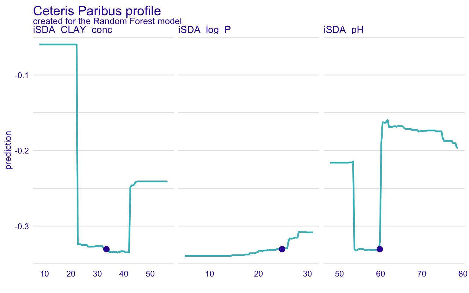
Figure 34: Ceteris paribus profiles for the Random Forest model, features; clay content, phosphorus concentration, pH
Show code
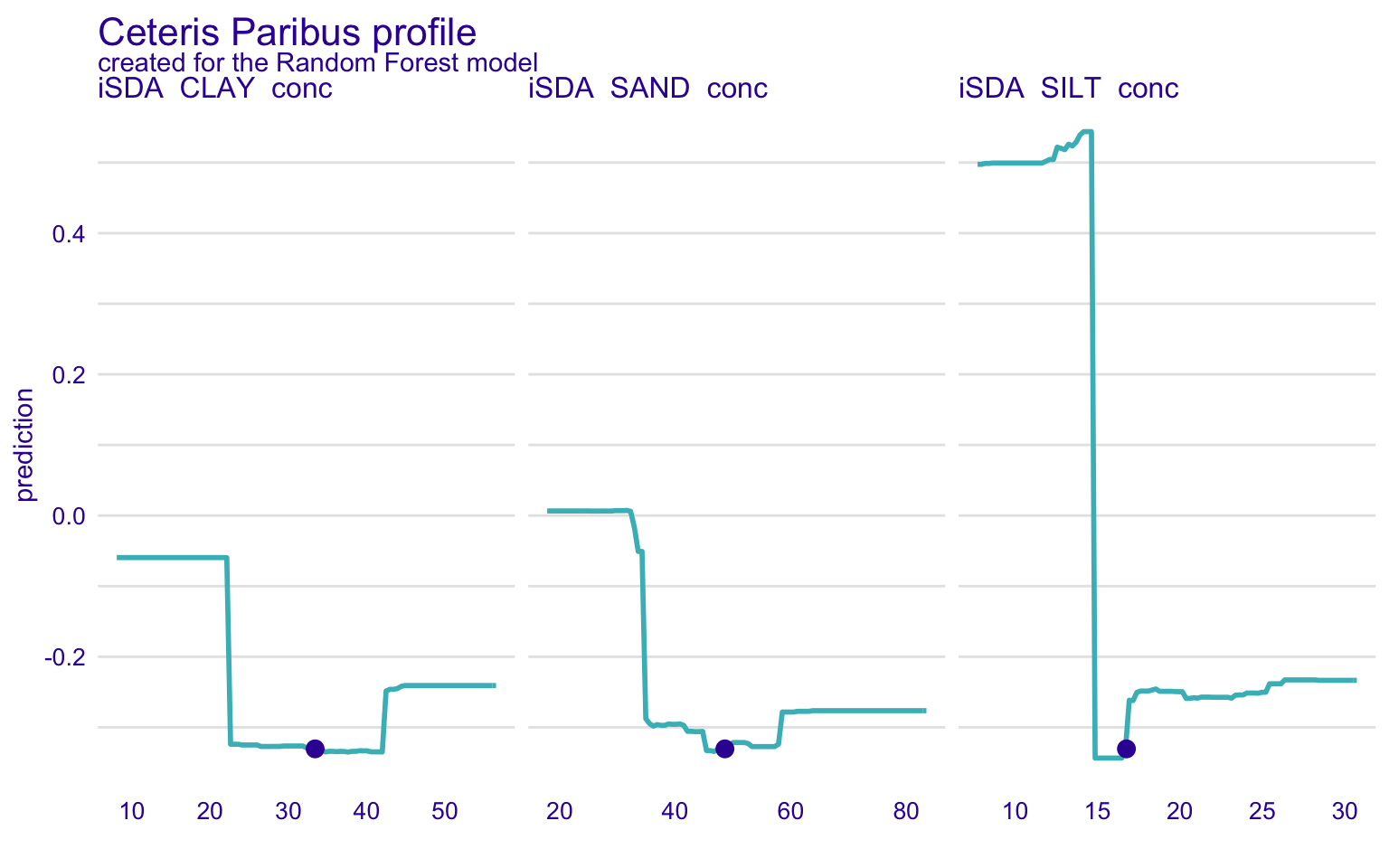
Figure 35: Ceteris paribus profiles for the Random Forest model, features; clay content, phosphorus concentration, pH
Show code
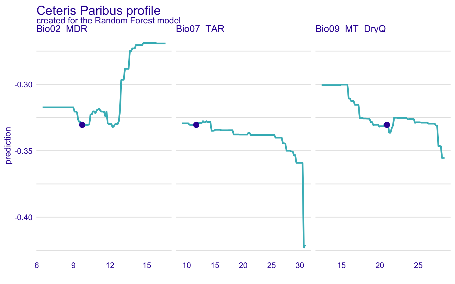
Figure 36: Ceteris paribus profiles for the Random Forest model, features; mean diurnal temperature range, temperature annual range and mean temperature of driest quarter
Show code
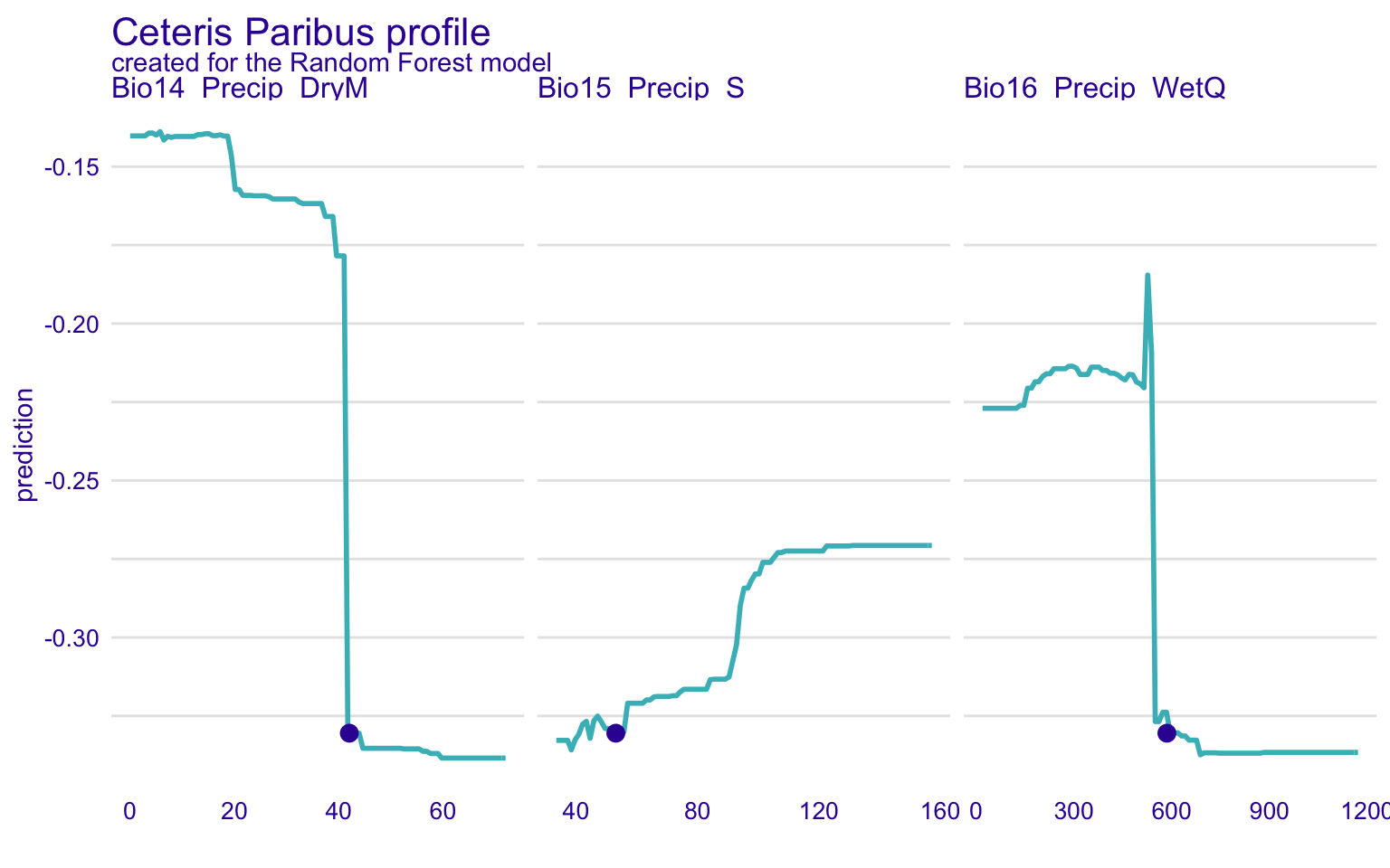
Figure 37: Ceteris paribus profiles for the Random Forest model, features; precipitation seasonality, precipitation driest month and precipitation wettest quarter
There are many intersting functionalities in ther DALEX package. Check out this website/blog for more inspiration on the DALEX package
STEP 19: Using the models to predict on new data
Let’s now try to use the models to predict on new data generated artificially from the training dataset. The expand_grid() function from the tidyr package is excellent for this. The function creates a tibble from all combinations of input data, hence it extrapolate the data. We will use this newly generated data to create Marginal Effect plots, therefore it is needed to keep a single feature while keeping all others constant.
First, removing NA from the predictor feature columns
af.train.wf %>%
  arrange()

old_data <- af.train.wf %>%
  rationalize() %>%
  drop_na()
Using expand_grid to generate new data from the traning data
Seven environmental predictor features are used to generate data for Marginal Effect plots. These predictors are having varied levels, while keeping all other features constant
Show code
# CLAY ------------------------------------------------------------------------
new_test_data_var_CLAY <-
  expand_grid(iSDA_CLAY_conc = c(10, 20, 30, 40),
            Site.Type = "Station",
            PrName = "Agroforestry Pruning",
            Out.SubInd = "Crop Yield",
            Product = "Maize",
            Tree = "Acacia albidam",
            Out.SubInd.Code = "CrY",
            Latitude = mean(old_data$Latitude),
            Longitude = mean(old_data$Longitude),
            Bio01_MT_Annu = mean(old_data$Bio01_MT_Annu),
            Bio02_MDR = mean(old_data$Bio02_MDR),
            Bio03_Iso = mean(old_data$Bio03_Iso),
            Bio04_TS = mean(old_data$Bio04_TS),
            Bio05_TWM = mean(old_data$Bio05_TWM),
            Bio06_MinTCM = mean(old_data$Bio06_MinTCM),
            Bio07_TAR = mean(old_data$Bio07_TAR),
            Bio08_MT_WetQ = mean(old_data$Bio08_MT_WetQ),
            Bio09_MT_DryQ = mean(old_data$Bio09_MT_DryQ),
            Bio10_MT_WarQ = mean(old_data$Bio10_MT_WarQ),
            Bio11_MT_ColQ = mean(old_data$Bio11_MT_ColQ),
            Bio12_Pecip_Annu = mean(old_data$Bio12_Pecip_Annu),
            Bio13_Precip_WetM = mean(old_data$Bio13_Precip_WetM),
            Bio14_Precip_DryM = mean(old_data$Bio14_Precip_DryM),
            Bio15_Precip_S = mean(old_data$Bio15_Precip_S),
            Bio16_Precip_WetQ = mean(old_data$Bio16_Precip_WetQ),
            Bio17_Precip_DryQ = mean(old_data$Bio17_Precip_DryQ),
            iSDA_Depth_to_bedrock = mean(old_data$iSDA_Depth_to_bedrock),
            iSDA_SAND_conc = mean(old_data$iSDA_SAND_conc),
            iSDA_SILT_conc = mean(old_data$iSDA_SILT_conc),
            iSDA_FE_Bulk_dens = mean(old_data$iSDA_FE_Bulk_dens),
            iSDA_log_C_tot = mean(old_data$iSDA_log_C_tot),
            iSDA_log_Ca = mean(old_data$iSDA_log_Ca),
            iSDA_log_eCEC = mean(old_data$iSDA_log_eCEC),
            iSDA_log_Fe = mean(old_data$iSDA_log_Fe),
            iSDA_log_K = mean(old_data$iSDA_log_K),
            iSDA_log_Mg = mean(old_data$iSDA_log_Mg),
            iSDA_log_N = mean(old_data$iSDA_log_N),
            iSDA_log_SOC = mean(old_data$iSDA_log_SOC),
            iSDA_log_P = mean(old_data$iSDA_log_P),
            iSDA_log_S = mean(old_data$iSDA_log_S),
            iSDA_pH = mean(old_data$iSDA_pH),
            ASTER_Altitude = mean(old_data$ASTER_Altitude),
            ASTER_Slope = mean(old_data$ASTER_Slope))

# SAND ------------------------------------------------------------------------
new_test_data_var_SAND <-
  expand_grid(iSDA_SAND_conc = c(50, 60, 70, 80),
            Site.Type = "Station",
            PrName = "Agroforestry Pruning",
            Out.SubInd = "Crop Yield",
            Product = "Maize",
            Tree = "Acacia albidam",
            Out.SubInd.Code = "CrY",
            Latitude = mean(old_data$Latitude),
            Longitude = mean(old_data$Longitude),
            Bio01_MT_Annu = mean(old_data$Bio01_MT_Annu),
            Bio02_MDR = mean(old_data$Bio02_MDR),
            Bio03_Iso = mean(old_data$Bio03_Iso),
            Bio04_TS = mean(old_data$Bio04_TS),
            Bio05_TWM = mean(old_data$Bio05_TWM),
            Bio06_MinTCM = mean(old_data$Bio06_MinTCM),
            Bio07_TAR = mean(old_data$Bio07_TAR),
            Bio08_MT_WetQ = mean(old_data$Bio08_MT_WetQ),
            Bio09_MT_DryQ = mean(old_data$Bio09_MT_DryQ),
            Bio10_MT_WarQ = mean(old_data$Bio10_MT_WarQ),
            Bio11_MT_ColQ = mean(old_data$Bio11_MT_ColQ),
            Bio12_Pecip_Annu = mean(old_data$Bio12_Pecip_Annu),
            Bio13_Precip_WetM = mean(old_data$Bio13_Precip_WetM),
            Bio14_Precip_DryM = mean(old_data$Bio14_Precip_DryM),
            Bio15_Precip_S = mean(old_data$Bio15_Precip_S),
            Bio16_Precip_WetQ = mean(old_data$Bio16_Precip_WetQ),
            Bio17_Precip_DryQ = mean(old_data$Bio17_Precip_DryQ),
            iSDA_Depth_to_bedrock = mean(old_data$iSDA_Depth_to_bedrock),
            iSDA_CLAY_conc = mean(old_data$iSDA_CLAY_conc),
            iSDA_SILT_conc = mean(old_data$iSDA_SILT_conc),
            iSDA_FE_Bulk_dens = mean(old_data$iSDA_FE_Bulk_dens),
            iSDA_log_C_tot = mean(old_data$iSDA_log_C_tot),
            iSDA_log_Ca = mean(old_data$iSDA_log_Ca),
            iSDA_log_eCEC = mean(old_data$iSDA_log_eCEC),
            iSDA_log_Fe = mean(old_data$iSDA_log_Fe),
            iSDA_log_K = mean(old_data$iSDA_log_K),
            iSDA_log_Mg = mean(old_data$iSDA_log_Mg),
            iSDA_log_N = mean(old_data$iSDA_log_N),
            iSDA_log_SOC = mean(old_data$iSDA_log_SOC),
            iSDA_log_P = mean(old_data$iSDA_log_P),
            iSDA_log_S = mean(old_data$iSDA_log_S),
            iSDA_pH = mean(old_data$iSDA_pH),
            ASTER_Altitude = mean(old_data$ASTER_Altitude),
            ASTER_Slope = mean(old_data$ASTER_Slope))


# SOIL pH  --------------------------------------------------------------------
new_test_data_iSDA_pH <-
  expand_grid(iSDA_pH = c(50, 60, 70, 80),
            Site.Type = "Station",
            PrName = "Agroforestry Pruning",
            Out.SubInd = "Crop Yield",
            Product = "Maize",
            Tree = "Acacia albida",
            Out.SubInd.Code = "CrY",
            Latitude = mean(old_data$Latitude),
            Longitude = mean(old_data$Longitude),
            Bio01_MT_Annu = mean(old_data$Bio01_MT_Annu),
            Bio02_MDR = mean(old_data$Bio02_MDR),
            Bio03_Iso = mean(old_data$Bio03_Iso),
            Bio04_TS = mean(old_data$Bio04_TS),
            Bio05_TWM = mean(old_data$Bio05_TWM),
            Bio06_MinTCM = mean(old_data$Bio06_MinTCM),
            Bio07_TAR = mean(old_data$Bio07_TAR),
            Bio08_MT_WetQ = mean(old_data$Bio08_MT_WetQ),
            Bio09_MT_DryQ = mean(old_data$Bio09_MT_DryQ),
            Bio10_MT_WarQ = mean(old_data$Bio10_MT_WarQ),
            Bio11_MT_ColQ = mean(old_data$Bio11_MT_ColQ),
            Bio12_Pecip_Annu = mean(old_data$Bio12_Pecip_Annu),
            Bio13_Precip_WetM = mean(old_data$Bio13_Precip_WetM),
            Bio14_Precip_DryM = mean(old_data$Bio14_Precip_DryM),
            Bio15_Precip_S = mean(old_data$Bio15_Precip_S),
            Bio17_Precip_DryQ = mean(old_data$Bio17_Precip_DryQ),
            Bio16_Precip_WetQ = mean(old_data$Bio16_Precip_WetQ),
            iSDA_Depth_to_bedrock = mean(old_data$iSDA_Depth_to_bedrock),
            iSDA_SAND_conc = mean(old_data$iSDA_SAND_conc),
            iSDA_CLAY_conc = mean(old_data$iSDA_CLAY_conc),
            iSDA_SILT_conc = mean(old_data$iSDA_SILT_conc),
            iSDA_FE_Bulk_dens = mean(old_data$iSDA_FE_Bulk_dens),
            iSDA_log_C_tot = mean(old_data$iSDA_log_C_tot),
            iSDA_log_Ca = mean(old_data$iSDA_log_Ca),
            iSDA_log_eCEC = mean(old_data$iSDA_log_eCEC),
            iSDA_log_Fe = mean(old_data$iSDA_log_Fe),
            iSDA_log_K = mean(old_data$iSDA_log_K),
            iSDA_log_Mg = mean(old_data$iSDA_log_Mg),
            iSDA_log_N = mean(old_data$iSDA_log_N),
            iSDA_log_SOC = mean(old_data$iSDA_log_SOC),
            iSDA_log_P = mean(old_data$iSDA_log_P),
            iSDA_log_S = mean(old_data$iSDA_log_S),
            ASTER_Altitude = mean(old_data$ASTER_Altitude),
            ASTER_Slope = mean(old_data$ASTER_Slope))


# PRECIPITATION SESONALITY --------------------------------------------------------------------
new_test_data_var_Precip_S <-
  expand_grid(Bio15_Precip_S = c(40, 50, 60, 70),
            Site.Type = "Station",
            PrName = "Agroforestry Pruning",
            Out.SubInd = "Crop Yield",
            Product = "Maize",
            Tree = "Acacia albida",
            Out.SubInd.Code = "CrY",
            Latitude = mean(old_data$Latitude),
            Longitude = mean(old_data$Longitude),
            Bio01_MT_Annu = mean(old_data$Bio01_MT_Annu),
            Bio02_MDR = mean(old_data$Bio02_MDR),
            Bio03_Iso = mean(old_data$Bio03_Iso),
            Bio04_TS = mean(old_data$Bio04_TS),
            Bio05_TWM = mean(old_data$Bio05_TWM),
            Bio06_MinTCM = mean(old_data$Bio06_MinTCM),
            Bio07_TAR = mean(old_data$Bio07_TAR),
            Bio08_MT_WetQ = mean(old_data$Bio08_MT_WetQ),
            Bio09_MT_DryQ = mean(old_data$Bio09_MT_DryQ),
            Bio10_MT_WarQ = mean(old_data$Bio10_MT_WarQ),
            Bio11_MT_ColQ = mean(old_data$Bio11_MT_ColQ),
            Bio12_Pecip_Annu = mean(old_data$Bio12_Pecip_Annu),
            Bio13_Precip_WetM = mean(old_data$Bio13_Precip_WetM),
            Bio14_Precip_DryM = mean(old_data$Bio14_Precip_DryM),
            Bio17_Precip_DryQ = mean(old_data$Bio17_Precip_DryQ),
            Bio16_Precip_WetQ = mean(old_data$Bio16_Precip_WetQ),
            iSDA_Depth_to_bedrock = mean(old_data$iSDA_Depth_to_bedrock),
            iSDA_SAND_conc = mean(old_data$iSDA_SAND_conc),
            iSDA_CLAY_conc = mean(old_data$iSDA_CLAY_conc),
            iSDA_SILT_conc = mean(old_data$iSDA_SILT_conc),
            iSDA_FE_Bulk_dens = mean(old_data$iSDA_FE_Bulk_dens),
            iSDA_log_C_tot = mean(old_data$iSDA_log_C_tot),
            iSDA_log_Ca = mean(old_data$iSDA_log_Ca),
            iSDA_log_eCEC = mean(old_data$iSDA_log_eCEC),
            iSDA_log_Fe = mean(old_data$iSDA_log_Fe),
            iSDA_log_K = mean(old_data$iSDA_log_K),
            iSDA_log_Mg = mean(old_data$iSDA_log_Mg),
            iSDA_log_N = mean(old_data$iSDA_log_N),
            iSDA_log_SOC = mean(old_data$iSDA_log_SOC),
            iSDA_log_P = mean(old_data$iSDA_log_P),
            iSDA_log_S = mean(old_data$iSDA_log_S),
            iSDA_pH = mean(old_data$iSDA_pH),
            ASTER_Altitude = mean(old_data$ASTER_Altitude),
            ASTER_Slope = mean(old_data$ASTER_Slope))

# PRECIPITATION DRIEST QUARTER --------------------------------------------------------------------
new_test_data_var_Precip_DryQ <-
  expand_grid(Bio17_Precip_DryQ = c(150, 180, 200, 220),
            Site.Type = "Station",
            PrName = "Agroforestry Pruning",
            Out.SubInd = "Crop Yield",
            Product = "Maize",
            Tree = "Acacia albida",
            Out.SubInd.Code = "CrY",
            Latitude = mean(old_data$Latitude),
            Longitude = mean(old_data$Longitude),
            Bio01_MT_Annu = mean(old_data$Bio01_MT_Annu),
            Bio02_MDR = mean(old_data$Bio02_MDR),
            Bio03_Iso = mean(old_data$Bio03_Iso),
            Bio04_TS = mean(old_data$Bio04_TS),
            Bio05_TWM = mean(old_data$Bio05_TWM),
            Bio06_MinTCM = mean(old_data$Bio06_MinTCM),
            Bio07_TAR = mean(old_data$Bio07_TAR),
            Bio08_MT_WetQ = mean(old_data$Bio08_MT_WetQ),
            Bio09_MT_DryQ = mean(old_data$Bio09_MT_DryQ),
            Bio10_MT_WarQ = mean(old_data$Bio10_MT_WarQ),
            Bio11_MT_ColQ = mean(old_data$Bio11_MT_ColQ),
            Bio12_Pecip_Annu = mean(old_data$Bio12_Pecip_Annu),
            Bio13_Precip_WetM = mean(old_data$Bio13_Precip_WetM),
            Bio14_Precip_DryM = mean(old_data$Bio14_Precip_DryM),
            Bio15_Precip_S = mean(old_data$Bio15_Precip_S),
            Bio16_Precip_WetQ = mean(old_data$Bio16_Precip_WetQ),
            iSDA_Depth_to_bedrock = mean(old_data$iSDA_Depth_to_bedrock),
            iSDA_SAND_conc = mean(old_data$iSDA_SAND_conc),
            iSDA_CLAY_conc = mean(old_data$iSDA_CLAY_conc),
            iSDA_SILT_conc = mean(old_data$iSDA_SILT_conc),
            iSDA_FE_Bulk_dens = mean(old_data$iSDA_FE_Bulk_dens),
            iSDA_log_C_tot = mean(old_data$iSDA_log_C_tot),
            iSDA_log_Ca = mean(old_data$iSDA_log_Ca),
            iSDA_log_eCEC = mean(old_data$iSDA_log_eCEC),
            iSDA_log_Fe = mean(old_data$iSDA_log_Fe),
            iSDA_log_K = mean(old_data$iSDA_log_K),
            iSDA_log_Mg = mean(old_data$iSDA_log_Mg),
            iSDA_log_N = mean(old_data$iSDA_log_N),
            iSDA_log_SOC = mean(old_data$iSDA_log_SOC),
            iSDA_log_P = mean(old_data$iSDA_log_P),
            iSDA_log_S = mean(old_data$iSDA_log_S),
            iSDA_pH = mean(old_data$iSDA_pH),
            ASTER_Altitude = mean(old_data$ASTER_Altitude),
            ASTER_Slope = mean(old_data$ASTER_Slope))

# TEMPERATURE MEAN DIURNAL RANGE  --------------------------------------------------------------------
new_test_data_var_MDR<-
  expand_grid(Bio02_MDR = c(12, 14, 16, 18),
            Site.Type = "Station",
            PrName = "Agroforestry Pruning",
            Out.SubInd = "Crop Yield",
            Product = "Maize",
            Tree = "Acacia albida",
            Out.SubInd.Code = "CrY",
            Latitude = mean(old_data$Latitude),
            Longitude = mean(old_data$Longitude),
            Bio01_MT_Annu = mean(old_data$Bio01_MT_Annu),
            Bio03_Iso = mean(old_data$Bio03_Iso),
            Bio04_TS = mean(old_data$Bio04_TS),
            Bio05_TWM = mean(old_data$Bio05_TWM),
            Bio06_MinTCM = mean(old_data$Bio06_MinTCM),
            Bio07_TAR = mean(old_data$Bio07_TAR),
            Bio08_MT_WetQ = mean(old_data$Bio08_MT_WetQ),
            Bio09_MT_DryQ = mean(old_data$Bio09_MT_DryQ),
            Bio10_MT_WarQ = mean(old_data$Bio10_MT_WarQ),
            Bio11_MT_ColQ = mean(old_data$Bio11_MT_ColQ),
            Bio12_Pecip_Annu = mean(old_data$Bio12_Pecip_Annu),
            Bio13_Precip_WetM = mean(old_data$Bio13_Precip_WetM),
            Bio14_Precip_DryM = mean(old_data$Bio14_Precip_DryM),
            Bio15_Precip_S = mean(old_data$Bio15_Precip_S),
            Bio17_Precip_DryQ = mean(old_data$Bio17_Precip_DryQ),
            Bio16_Precip_WetQ = mean(old_data$Bio16_Precip_WetQ),
            iSDA_Depth_to_bedrock = mean(old_data$iSDA_Depth_to_bedrock),
            iSDA_SAND_conc = mean(old_data$iSDA_SAND_conc),
            iSDA_CLAY_conc = mean(old_data$iSDA_CLAY_conc),
            iSDA_SILT_conc = mean(old_data$iSDA_SILT_conc),
            iSDA_FE_Bulk_dens = mean(old_data$iSDA_FE_Bulk_dens),
            iSDA_log_C_tot = mean(old_data$iSDA_log_C_tot),
            iSDA_log_Ca = mean(old_data$iSDA_log_Ca),
            iSDA_log_eCEC = mean(old_data$iSDA_log_eCEC),
            iSDA_log_Fe = mean(old_data$iSDA_log_Fe),
            iSDA_log_K = mean(old_data$iSDA_log_K),
            iSDA_log_Mg = mean(old_data$iSDA_log_Mg),
            iSDA_log_N = mean(old_data$iSDA_log_N),
            iSDA_log_SOC = mean(old_data$iSDA_log_SOC),
            iSDA_log_P = mean(old_data$iSDA_log_P),
            iSDA_log_S = mean(old_data$iSDA_log_S),
            iSDA_pH = mean(old_data$iSDA_pH),
            ASTER_Altitude = mean(old_data$ASTER_Altitude),
            ASTER_Slope = mean(old_data$ASTER_Slope))


# TEMPERATURE OF WETTEST MONTH --------------------------------------------------------------------
new_test_data_var_TWM <-
  expand_grid(Bio05_TWM = c(20, 25, 30, 35),
            Site.Type = "Station",
            PrName = "Agroforestry Pruning",
            Out.SubInd = "Crop Yield",
            Product = "Maize",
            Tree = "Acacia albida",
            Out.SubInd.Code = "CrY",
            Latitude = mean(old_data$Latitude),
            Longitude = mean(old_data$Longitude),
            Bio01_MT_Annu = mean(old_data$Bio01_MT_Annu),
            Bio02_MDR = mean(old_data$Bio02_MDR),
            Bio03_Iso = mean(old_data$Bio03_Iso),
            Bio04_TS = mean(old_data$Bio04_TS),
            Bio06_MinTCM = mean(old_data$Bio06_MinTCM),
            Bio07_TAR = mean(old_data$Bio07_TAR),
            Bio08_MT_WetQ = mean(old_data$Bio08_MT_WetQ),
            Bio09_MT_DryQ = mean(old_data$Bio09_MT_DryQ),
            Bio10_MT_WarQ = mean(old_data$Bio10_MT_WarQ),
            Bio11_MT_ColQ = mean(old_data$Bio11_MT_ColQ),
            Bio12_Pecip_Annu = mean(old_data$Bio12_Pecip_Annu),
            Bio13_Precip_WetM = mean(old_data$Bio13_Precip_WetM),
            Bio14_Precip_DryM = mean(old_data$Bio14_Precip_DryM),
            Bio15_Precip_S = mean(old_data$Bio15_Precip_S),
            Bio17_Precip_DryQ = mean(old_data$Bio17_Precip_DryQ),
            Bio16_Precip_WetQ = mean(old_data$Bio16_Precip_WetQ),
            iSDA_Depth_to_bedrock = mean(old_data$iSDA_Depth_to_bedrock),
            iSDA_SAND_conc = mean(old_data$iSDA_SAND_conc),
            iSDA_CLAY_conc = mean(old_data$iSDA_CLAY_conc),
            iSDA_SILT_conc = mean(old_data$iSDA_SILT_conc),
            iSDA_FE_Bulk_dens = mean(old_data$iSDA_FE_Bulk_dens),
            iSDA_log_C_tot = mean(old_data$iSDA_log_C_tot),
            iSDA_log_Ca = mean(old_data$iSDA_log_Ca),
            iSDA_log_eCEC = mean(old_data$iSDA_log_eCEC),
            iSDA_log_Fe = mean(old_data$iSDA_log_Fe),
            iSDA_log_K = mean(old_data$iSDA_log_K),
            iSDA_log_Mg = mean(old_data$iSDA_log_Mg),
            iSDA_log_N = mean(old_data$iSDA_log_N),
            iSDA_log_SOC = mean(old_data$iSDA_log_SOC),
            iSDA_log_P = mean(old_data$iSDA_log_P),
            iSDA_log_S = mean(old_data$iSDA_log_S),
            iSDA_pH = mean(old_data$iSDA_pH),
            ASTER_Altitude = mean(old_data$ASTER_Altitude),
            ASTER_Slope = mean(old_data$ASTER_Slope))
Predicting with the Random Forest model on the new data
pred_new_data_CLAY <- predict(rf_best_race_trained_wf,
                      new_data = new_test_data_var_CLAY)

pred_new_data_SAND <- predict(rf_best_race_trained_wf,
                      new_data = new_test_data_var_SAND)

pred_new_data_pH <- predict(rf_best_race_trained_wf,
                      new_data = new_test_data_iSDA_pH)

pred_new_data_Precip_S <- predict(rf_best_race_trained_wf,
                      new_data = new_test_data_var_Precip_S)

pred_new_data_Precip_DryQ <- predict(rf_best_race_trained_wf,
                      new_data = new_test_data_var_Precip_DryQ)

pred_new_data_MDR <- predict(rf_best_race_trained_wf,
                      new_data = new_test_data_var_MDR)

pred_new_data_TWM <- predict(rf_best_race_trained_wf,
                      new_data = new_test_data_var_TWM)

# We get a few warnings we can ignore
# Warning: Novel levels found in column 'Tree': 'Acacia albidam'. The levels have been removed, and values have been coerced to 'NA'.
# Warning: Novel levels found in column 'Tree': 'Acacia albidam'. The levels have been removed, and values have been coerced to 'NA'.
Creating the dataset of predicted response ratio values for each of the predictors
These dataframes/tibbles will be used to generate ggplots of marginal effects for each of the variables.
Show code
pred_new_data_CLAY <- tibble(iSDA_CLAY_conc = c(10, 20, 30, 40),
                          .pred = c(0.5355357, 0.5281725, 0.4982191, 0.5128507))

pred_new_data_SAND <- tibble(iSDA_SAND_conc = c(50, 60, 70, 80),
                          .pred = c(0.4994193, 0.4955434, 0.5159416, 0.5159416))

pred_new_data_pH <- tibble(iSDA_pH = c(50, 60, 70, 80),
                          .pred = c(0.5760564  , 0.4931747, 0.4762354, 0.4695003))

pred_new_data_Precip_S <- tibble(Bio15_Precip_S = c(40, 50, 60, 70),
                          .pred = c(0.5320894  , 0.5322152, 0.5507409, 0.4489401))

pred_new_data_Precip_DryQ <- tibble(Bio17_Precip_DryQ = c(150, 180, 200, 220),
                          .pred = c(0.5352552  , 0.5333205, 0.5294350, 0.5294350))

pred_new_data_MDR <- tibble(Bio02_MDR = c(12, 14, 16, 18),
                          .pred = c(0.4648982  , 0.4637734, 0.4791219, 0.4791219))

pred_new_data_TWM <- tibble(Bio05_TWM = c(20, 25, 30, 35),
                          .pred = c(0.4372342  , 0.4372342, 0.4981338, 0.3629274))


# SAVING THE PREDICTED DATASETS FOR EACH OF THE PREDICTOR FEATURES

saveRDS(pred_new_data_CLAY, here::here("TidyModWflSet_OUTPUT","pred_new_data_CLAY.RDS"))
saveRDS(pred_new_data_SAND, here::here("TidyModWflSet_OUTPUT","pred_new_data_SAND.RDS"))
saveRDS(pred_new_data_pH, here::here("TidyModWflSet_OUTPUT","pred_new_data_pH.RDS"))

saveRDS(pred_new_data_Precip_S, here::here("TidyModWflSet_OUTPUT","pred_new_data_Precip_S.RDS"))
saveRDS(pred_new_data_Precip_DryQ, here::here("TidyModWflSet_OUTPUT","pred_new_data_Precip_DryQ.RDS"))

saveRDS(pred_new_data_MDR, here::here("TidyModWflSet_OUTPUT","pred_new_data_MDR.RDS"))
saveRDS(pred_new_data_TWM, here::here("TidyModWflSet_OUTPUT","pred_new_data_TWM.RDS"))
Show code
pred_new_data_CLAY <- cpp_newObs_1_rf <-  readRDS(here::here("TidyModWflSet_OUTPUT","pred_new_data_CLAY.RDS"))


ggplot(pred_new_data_CLAY, aes(x =iSDA_CLAY_conc, y = .pred)) +
  geom_line(alpha = .5, lty = 2, size = 2, col = "darkorange") +
  geom_point(size = 4) +
  theme_bw() +
  ggtitle("CLAY: Marginal effect plot") +
  ylab("Predicted response ratio") +
  xlab("Clay content")
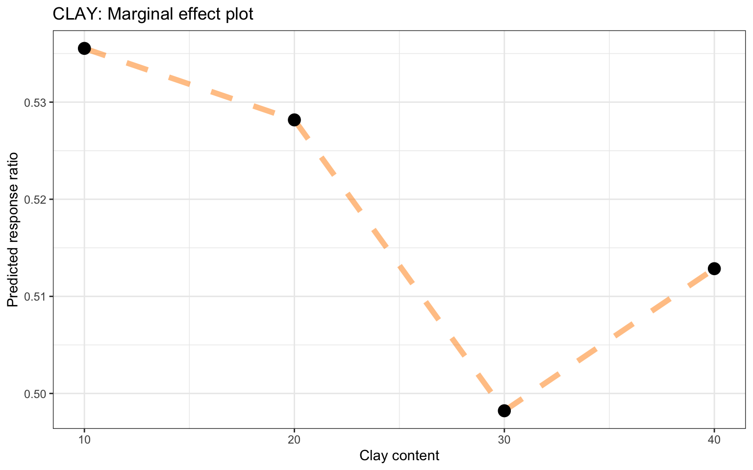
Figure 38: Marginal effects plot for clay content based on the RF model
Show code
pred_new_data_SAND <- cpp_newObs_1_rf <-  readRDS(here::here("TidyModWflSet_OUTPUT","pred_new_data_SAND.RDS"))

ggplot(pred_new_data_SAND, aes(x =iSDA_SAND_conc, y = .pred)) +
  geom_line(alpha = .5, lty = 2, size = 2, col = "darkorange") +
  geom_point(size = 4) +
  theme_bw() +
  ggtitle("SAND: Marginal effect plot") +
  ylab("Predicted response ratio") +
  xlab("Sand content")
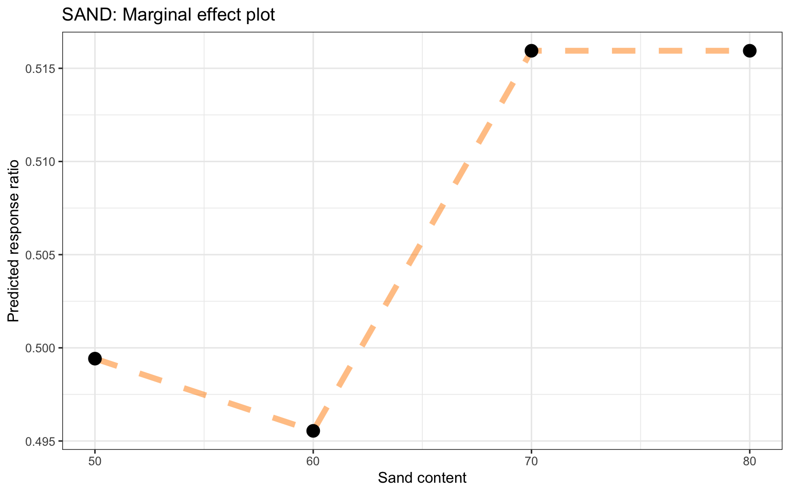
Figure 39: Marginal effects plot for sand content based on the RF model
Show code
pred_new_data_pH <- cpp_newObs_1_rf <-  readRDS(here::here("TidyModWflSet_OUTPUT","pred_new_data_pH.RDS"))

ggplot(pred_new_data_pH, aes(x =iSDA_pH, y = .pred)) +
  geom_line(alpha = .5, lty = 2, size = 2, col = "darkorange") +
  geom_point(size = 4) +
  theme_bw() +
  ggtitle("Soil pH: Marginal effect plot") +
  ylab("Predicted response ratio") +
  xlab("pH")
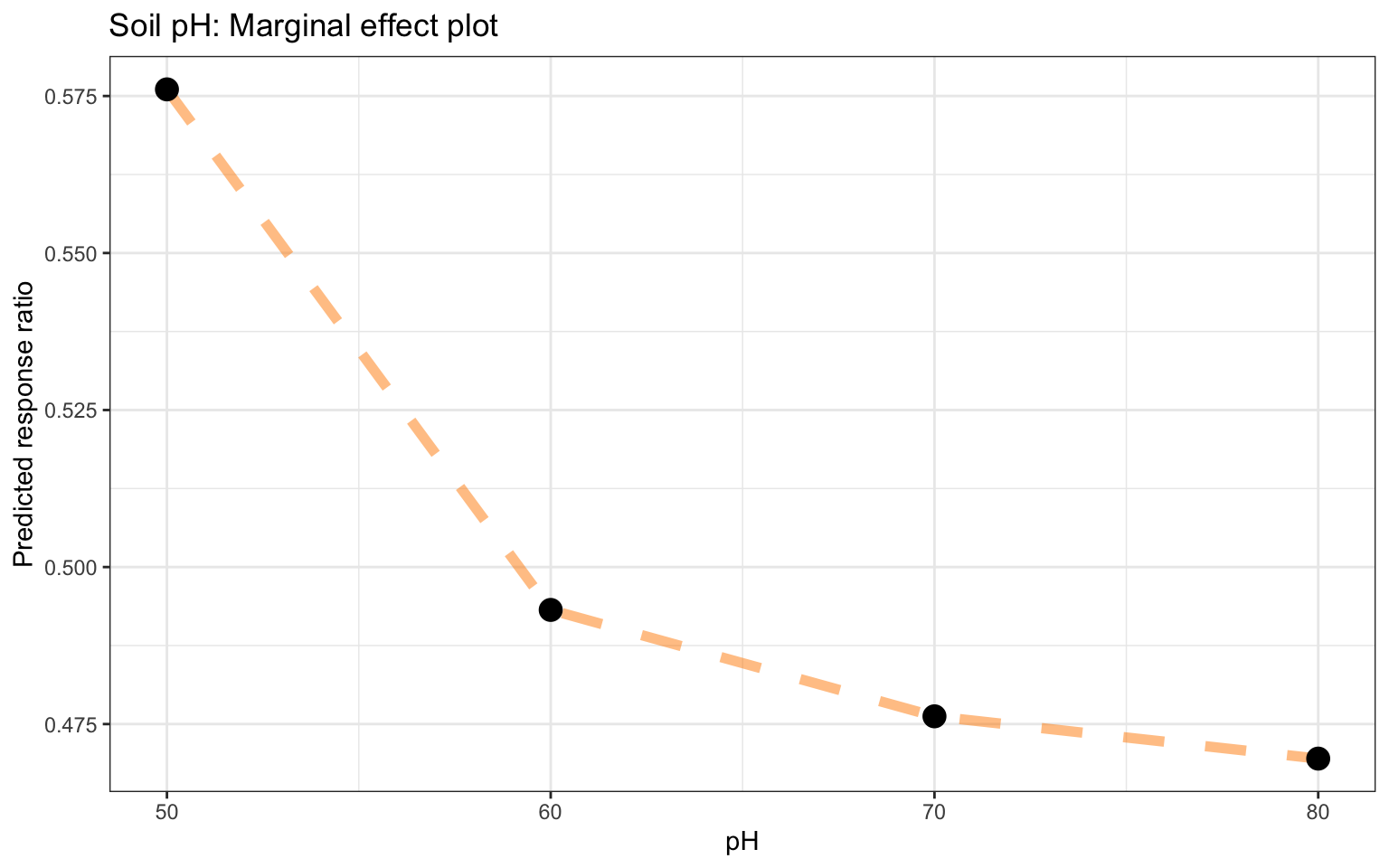
Figure 40: Marginal effects plot for pH based on the RF model
Show code
pred_new_data_Precip_S <- cpp_newObs_1_rf <-  readRDS(here::here("TidyModWflSet_OUTPUT","pred_new_data_Precip_S.RDS"))

ggplot(pred_new_data_Precip_S, aes(x = Bio15_Precip_S, y = .pred)) +
  geom_line(alpha = .5, lty = 2, size = 2, col = "midnightblue") +
  geom_point(size = 4) +
  theme_bw() +
  ggtitle("Precipitation (Seasonal): Marginal effect plot") +
  ylab("Predicted response ratio") +
  xlab("Precipitation (Seasonal)")
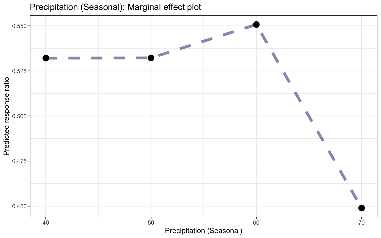
Figure 41: Marginal effects plot for precipitation seasonality based on the RF model
Show code
pred_new_data_Precip_DryQ <- readRDS(here::here("TidyModWflSet_OUTPUT","pred_new_data_Precip_DryQ.RDS"))

ggplot(pred_new_data_Precip_DryQ, aes(x =Bio17_Precip_DryQ, y = .pred)) +
  geom_line(alpha = .5, lty = 2, size = 2, col = "midnightblue") +
  geom_point(size = 4) +
  theme_bw() +
  ggtitle("Precipitation (Driest Quarter): Marginal effect plot") +
  ylab("Predicted response ratio") +
  xlab("Precipitation (Driest Quarter)")
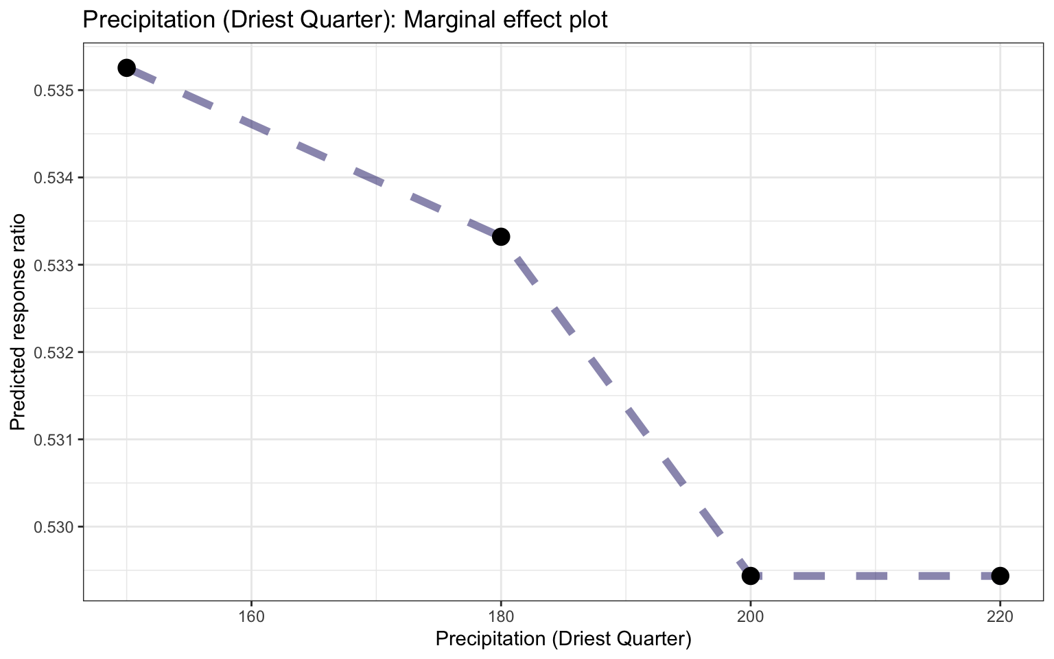
Figure 42: Marginal effects plot for precipitation of driest quarter based on the RF model
Show code
pred_new_data_MDR <- readRDS(here::here("TidyModWflSet_OUTPUT","pred_new_data_MDR.RDS"))

ggplot(pred_new_data_MDR, aes(x =Bio02_MDR, y = .pred)) +
  geom_line(alpha = .5, lty = 2, size = 2, col = "darkgreen") +
  geom_point(size = 4) +
  theme_bw() +
  ggtitle("Temperature (Mean Diurnal Range): Marginal effect plot") +
  ylab("Predicted response ratio") +
  xlab("Temperature (Mean Diurnal Range)")
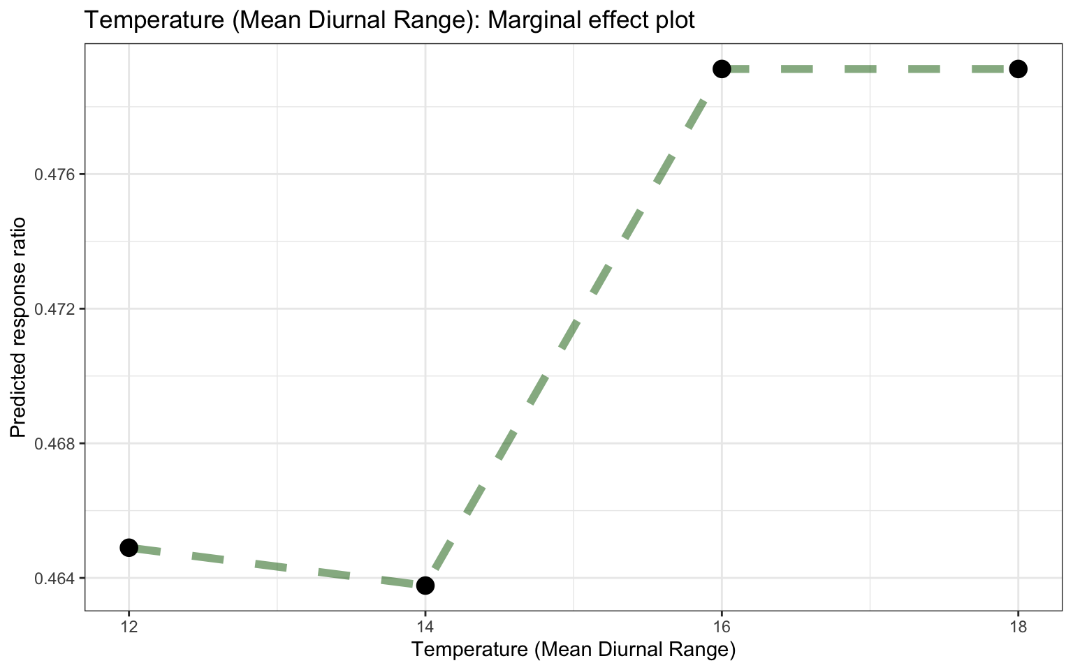
Figure 43: Marginal effects plot for temperature mean diurnal range based on the RF model
Show code
pred_new_data_TWM <- readRDS(here::here("TidyModWflSet_OUTPUT","pred_new_data_TWM.RDS"))


ggplot(pred_new_data_TWM, aes(x = Bio05_TWM, y = .pred)) +
  geom_line(alpha = .5, lty = 2, size = 2, col = "darkgreen") +
  geom_point(size = 4) +
  theme_bw() +
  ggtitle("Temperature (Max of Warmest Month): Marginal effect plot") +
  ylab("Predicted response ratio") +
  xlab("Temperature (Max of Warmest Month)")
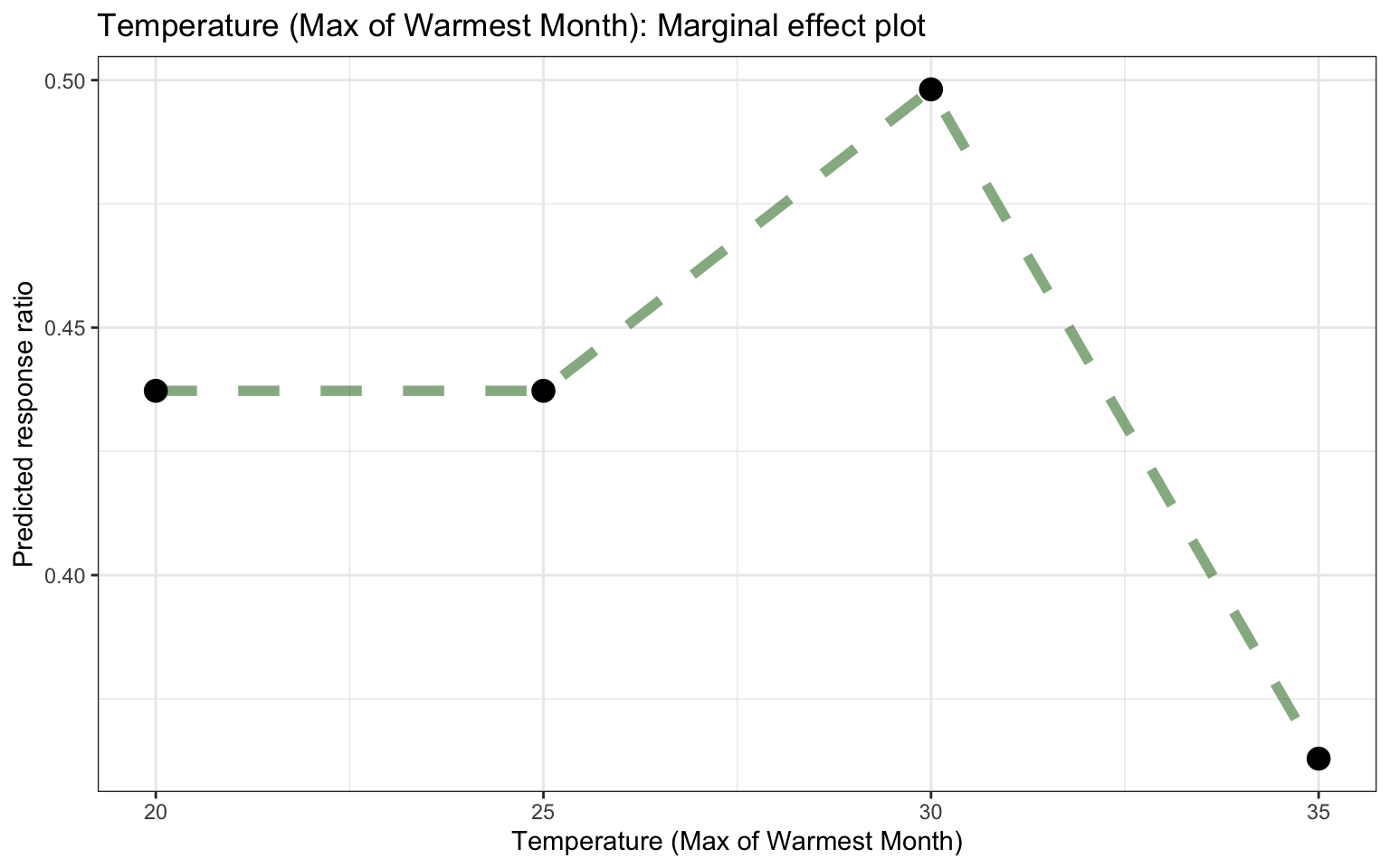
Figure 44: Marginal effects plot for temperature of warmest month based on the RF model